This post delves into a disagreement I have with three prominent political scientists, Jens Hainmueller, Jonathan Mummolo, and Yiqing Xu (HMX), on a fundamental methodological question: how to analyze interactions in observational data?
In 2019, HMX proposed the "binning estimator" for studying interactions, a technique that is now commonly used by political scientists. I argued in Colada[121] that with observational data the binning estimator was too often biased. HMX disagreed (.pdf).
What's behind our disagreement? In a nutshell, you are.
With HMX we disagree on what is the question you want to answer when you analyze interactions.
The specific disagreement is that while I believe researchers want to probe interactions under ceteris paribus, HMX do not.
Estimands
HMX write "we show that once the estimand is properly defined, the critiques . . . no longer hold" (p.5).
Estimand is the target quantity of estimation. For example, the estimand can be the population mean, and the estimator the sample mean. In this case the estimand is what you are trying to estimate when probing the interaction. HMX are saying, paraphrasing, "the binning estimator may miss the estimand Uri has in mind, but not the one we have in mind".
Researchers are free to ask whatever question they want, but, that question determines the appropriate estimand to set. On the one hand, this means there are no intrinsically wrong estimands. On the other hand, it means that there are estimands that are wrong for a given question. A dictionary isn’t right or wrong as a book, but it’s the wrong book if you’re looking for a waffle recipe.
I think the estimand HMX use to defend the binning estimator is wrong in that way; it does not inform the question I think people have when studying interactions. Specifically, I think political scientists ask questions under ceteris paribus, but the estimand HMX chose reflects a question asked without ceteris paribus.
In this post I use a concrete example, PhD admissions, to go over the binning estimator and the shortcomings I identified in Colada[121]. I then return to the issue of choosing the estimand.
PhD admissions example
Imagine a PhD admissions committee, where a few professors are tasked with reviewing 100s of applications, rating each applicant on a 0-7 scale. The professors take a shortcut: they don't read the applications. Instead, they take each applicant's GRE score, and submit log(GRE) as the applicant's rating. Let's say GRE scores are 1-1000. If an applicant has a GRE of 1000, the profs compute log(1000)=6.9, and submit that as the rating (see Figure 1).
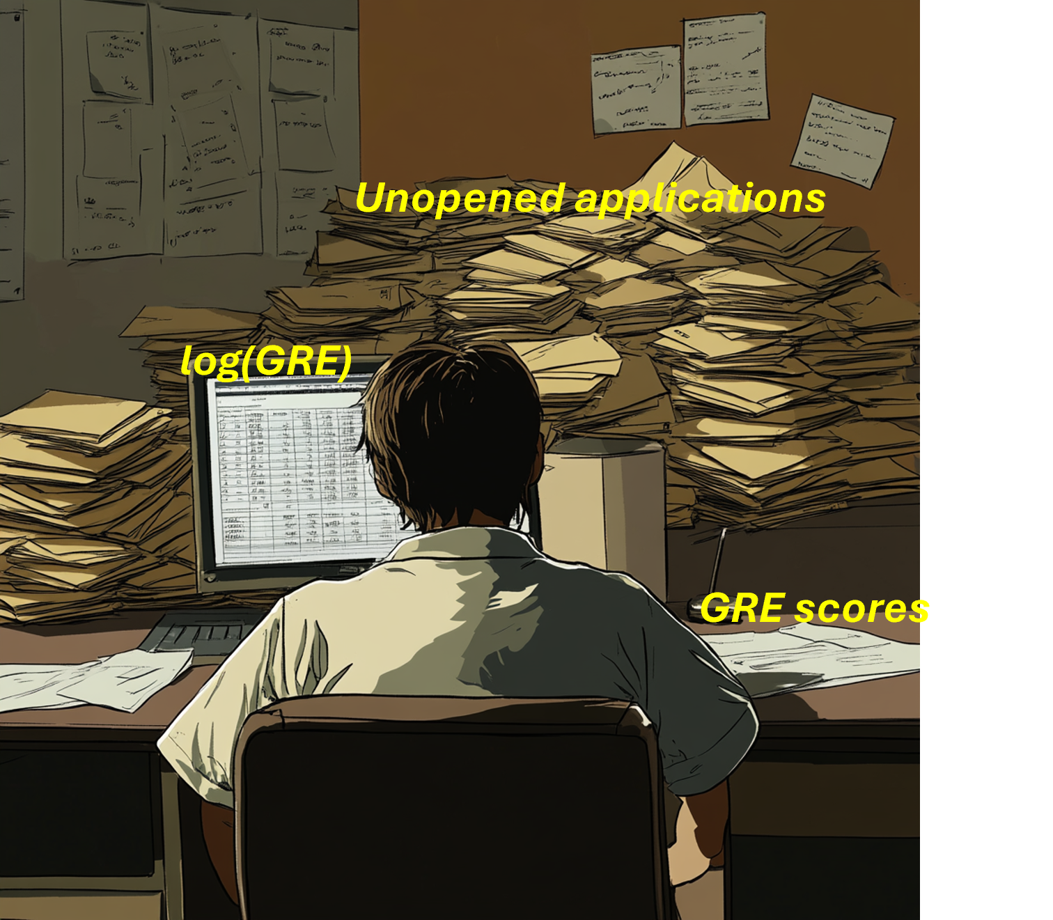
Fig 1. A professor evaluating PhD applications based solely on GRE scores.
These 0-7 ratings are then emailed to Alex, the department chair, who makes final admissions decisions.
Alex had given the committee a clear instruction: "Please make sure to take into account how much research experience applicants have when using their GRE scores to arrive at an overall rating".
We, as omniscient readers, know the profs didn't follow that instruction. They couldn't possibly have taken experience into account because the profs didn't open the files and didn't know applicants' research experience. They just entered log(GRE). But Alex, our protagonist, doesn't know that.
Alex gets data
Alex, however, is a social scientist, and figures that with a little regression it is easy to check whether the instructions were followed. All that is needed is checking whether there is a significant GRE×research interaction when predicting the 0-7 ratings.
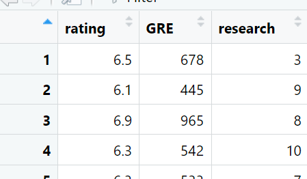
Alex asks some RAs to evaluate the research experience for every applicant on a 0-10 scale. The resulting dataset looks like this:
Before running the desired regression, Alex does some descriptive stats and notices that GRE and research experience are positively correlated, see Figure 2. That makes sense. Undergrads who are keener on grad school prepare more for the GRE and work as research assistants, producing the positive association. This fact will be important in our story.

Fig 2. GRE and research experience are correlated
Alex then runs this regression: rating = a + b·GRE + c·research + d·GRE×research,
finding a significant negative interaction:
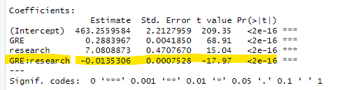
Note: to make things more readable I multiplied the DV, the 0-7 ratings, by 100. E.g., the intercept is 4.63, not 463.
Alex concludes that the committee did take into account research experience. The more research experience applicants had, the less the GRE mattered. Omniscient reader: remember that this is wrong. The reality is that rating=log(GRE) for any research experience level.
The interaction is negative because it is picking up the nonlinearity of GRE. More generally, when x and z in the x·z interaction are correlated, the interaction is biased by any nonlinearity in the effect of x or z (see Simonsohn 2024; Ganzach 1997).
What does the binning estimator say?
Conveniently for our purposes, Alex is a political scientist and knows that HMX recommend running the binning estimator after a regression with an interaction, to diagnose possible non-linearities. Alex loads HMX's 'interflex' R package and produces the figure below.
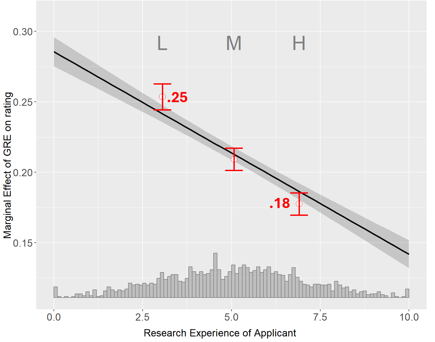
Fig 3. Binning estimator output from HMX's {interflex} package.
Red numbers added for this post.
On the x-axis we have the moderator, research experience, and its distribution.
On the y-axis we have the marginal effect of GRE, the increase in a candidate's rating when their GRE score increases by 1 point. The figure shows that the marginal effect fluctuates in the .15 to .30 range.
Inside the graph we have a straight line and three red confidence intervals.
The straight line depicts the marginal effect implied by the regression from the previous section:
Specifically, marginal effect = b + d×experience = 0.288 -.0135*experience.
(dear psychologists: that's the Johnson-Neyman line)
Lastly, the three red confidence intervals are the binning estimator. The data were split into three bins with low, medium and high moderator values, and the marginal effect of GRE was computed within each bin. The three red confidence intervals show that as we increase experience, from the low bin to the high bin, we see the marginal effect of GRE drop substantially from 0.25 to 0.18. In English: as was the case with the linear regression, the binning estimator seems to erroneously suggest that for applicants with more experience the GRE matters a lot less.
Alex knows that the key thing HMX said to check was whether the red confidence intervals line up with the regression's line. They do. Alex closes the laptop feeling assured the committee did as instructed. (But don't forget, Alex is wrong).
Why is the binning estimator getting this wrong?
In Colada[121] I explained the problem as an instance of omitted variable bias. But given this post's emphasis on the research question determining the right estimand, here I will explain it a bit differently. I will rely on the notion of ceteris paribus, showing that the binning estimator violates it.
Let's build an understanding with Figure 4, which reprints two figures you already saw, with added yellow tags.
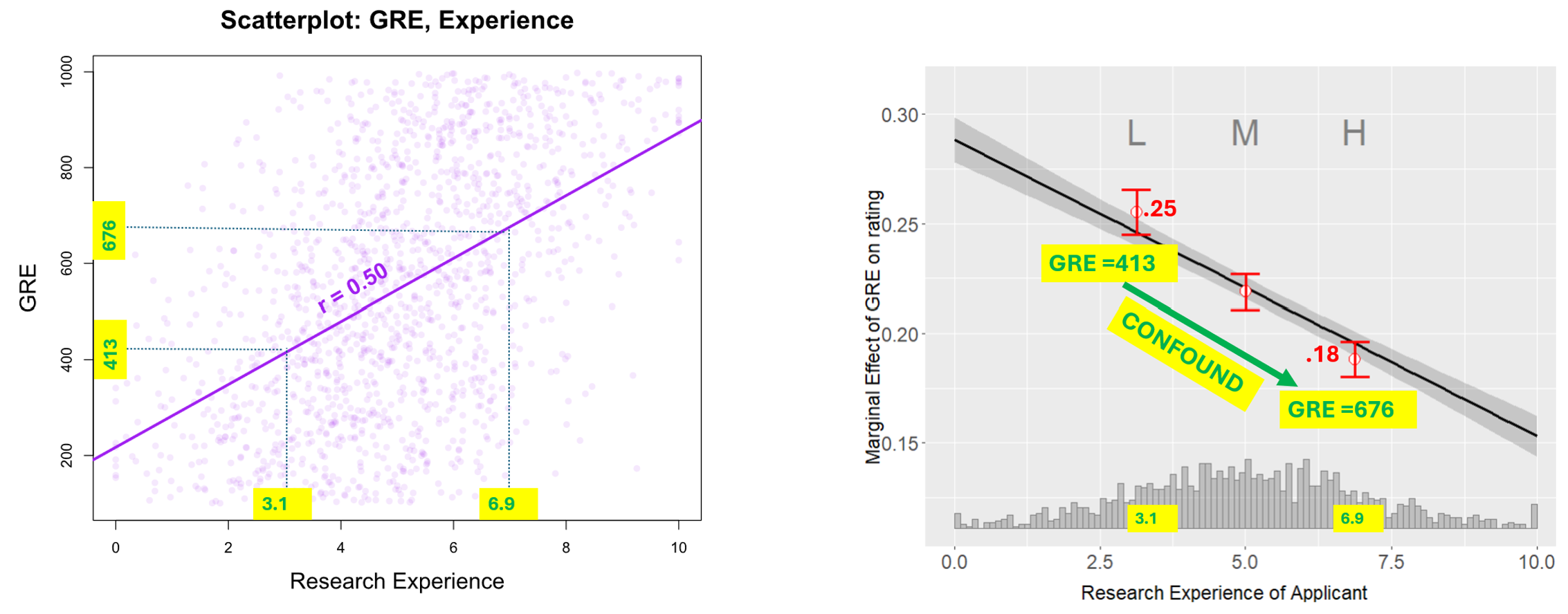
Fig 4. Comparing across bins we change both research experience and GRE
The left chart shows that because GRE and research experience are correlated, moving from Low to High research experience implies also moving from low to high GRE scores.
Therefore, when in the right chart, in the binning estimator, we compare the Low bin with the High bin, we compare applications that have different research experience levels (M=3.1 vs M= 6.9) but also different GRE levels (M=413 vs M=676). Because rating=log(GRE), the marginal effect is 1/GRE, thus higher GRE→lower marginal effect. Making comparisons while changing two variables at once is a no-no, it violates ceteris paribus, you cannot infer where the change is coming from. (Here as omniscient readers we know that the entirety of the difference between L and H is driven by GRE levels, and has nothing to do with the moderator per-se).
Note: if the true model were linear, violating ceteris paribus would be inconsequential because the marginal effect of GRE would not change with different GRE levels.
Getting it wrong in the opposite way
Perhaps thinking of a case where the binning estimator gives the opposite result for the same true model will help. Let's say there are two types of applicants: American & Foreign. American applicants have r(GRE, experience)>0, as before. But foreign applicants have a negative correlation, perhaps because abroad, the undergrads doing RA work are those who need money the most, and those students have less access to resources to prep the GRE.
Still every applicant, American or Foreign, got rated as log(GRE) and research experience didn't matter.
But check out what the binning estimator will show:
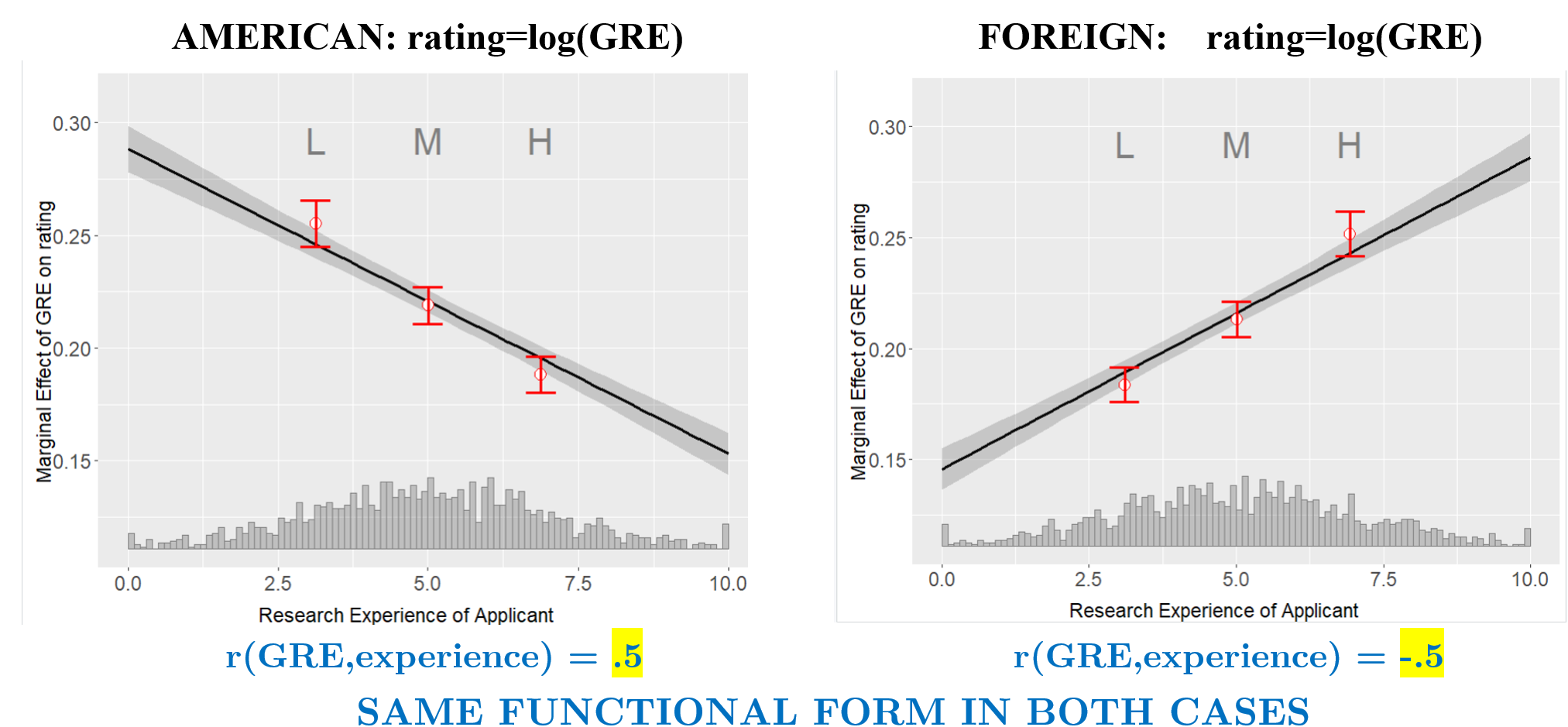 Fig 5. Spurious interactions in binning estimator can reverse with same true functional format
The intuition for the upward slope for foreigners is the same as the negative one for Americans. As we go left-to-right from L to H, we are increasing research, but simultaneously decreasing the GRE, and the lower the GRE, the higher the benefit of an extra GRE point.
HMX response: the binning estimator isn't biased for the estimand researchers want
HMX do not dispute that the binning estimator confounds changes caused by the moderator (e.g. experience) with changes caused by the focal variable (e.g., GRE).1For example, in page 8 in their response, they consider my example where the true model is y=x2 – 0.5·x and there is also a confounder, variable z correlated with x but not in the true model (z is a confounder through x·z, because x·z is correlated with omitted x2). HMX nevertheless define the estimand for the marginal effect of x a as ∂y /∂x = z – .5. That is, they build into the estimand the association between x and z, so that when considering different z values, x is allowed to vary freely, rather than keep it constant per ceteris paribus. If you keep x constant, changes in z have no association with changes in y. The estimand they consider thus also violates ceteris paribus. But, they think of it as a feature, while I think of it as a bug. HMX propose that researchers want an estimator that, when comparing applicants with high vs low research experience, will also change the underlying GRE.
Here are the two research questions we are considering.
Question 1. Does research experience correlate with the marginal effect of GRE?" (ceteris paribus)
Question 2. Does research experience correlate with the marginal effect of GRE?" (without ceteris paribus)
Uri thinks you want to ask Q1, HMX that you want to ask Q2 (or at least they act as if they believe that).
This figure shows the connection between the question being asked and the estimands.

Fig 6. How the question shapes the estimand.
The left chart has the marginal effect of GRE on the 0-7 rating (∂rating/∂GRE=1/GRE). As before, I multiply by 100 to make numbers easy to read.
The middle chart shows that if we keep GRE level constant, there is no correlation between the marginal effect of the GRE and research experience. The estimand's true population value here is 0, ∂rating/∂GRE does not depend on research experience. (GAM Johnson Neyman recovers this estimand, see #7 in R Code).
The right plot shows that if we do not keep GRE constant, and instead, we change GRE based on the association it happens to have in the data with the moderator, the true population value of the estimand has a population value that's not zero. Instead it is the average of the change in marginal effect of GRE across different GRE levels plus a possible interaction effect. This is what HMX's tools, the binning and kernel estimator recover.
Relevant papers?
I haven't found discussions of this ceteris paribus issue in relation to probing interactions or computing average marginal effects more generally; if you know of relevant articles or posts let me know. The closest I know is by Greene (2010 .htm), the author of a famed PhD level econometrics textbook, who argues that averaging marginal effects across predictor values in a non-linear interaction model (as the estimand and estimators chosen by HMX do) leads to "generally uninformative and sometimes contradictory and misleading results" (p. 295).
![]()
R Code to reproduce all figures
Author feedback
Our policy (.htm) is to share drafts of blog posts with authors whose work we discuss, in order to solicit suggestions for things we should change prior to posting. The goal of this policy is to openly debate things in private before posting, avoiding errors of substance or tone. I did not share the draft of this post with HMX because I repeatedly tried and failed to engage with them in debate. First, they only told me of their response after they posted it to arxiv (not reciprocating me having shared the post with them weeks in advance). Then they insisted I add a link to it from my previous post before giving me a chance to read it (it's 26 pages long). I did. I then proposed we have an open exchange to understand our different points of views, I sent several question to them, they were not answered. As I read their response I started thinking about the ceteris paribus issue addressed in this post and I asked them about it. They asked that I provide a formal treatment of the issue, I did. I sent them a 5 page document. They did not reply to that either. As I drafted this post I asked them again whether they agree that their estimand violates ceteris paribus, they replied that they had to "agree to disagree" a phrase which does not apply to a situation where you have not explained to your counterpart what your position is (and your counterpart was not asked whether they also agree to disagree, in takes two to agree). After that response I gave up trying to have a dialogue with HMX, and decided to just go ahead and post.
They have not had the worst reaction to a post I have written, they would need to sue me for at least $25,000,001 to earn that position, but they are tied in second place with 3 other hostile groups of authors. All of them methodologists. I think there is something interesting there. You would think that those of us who keep telling everyone how to do their research would be especially open to debating someone disagreeing with what what we are saying. But my anecdotal evidence suggests lower tolerance to criticisms in such group.
I did share drafts and received feedback from five other researchers. Thanks!