Behavioral scientists have put forth evidence that the weather affects all sorts of things, including the stock market, restaurant tips, car purchases, product returns, art prices, and college admissions.
It is not easy to properly study the effects of weather on human behavior. This is because weather is (obviously) seasonal, as is much of what people do. This means that any investigation of the relation between weather and behavior must properly control for seasonality.
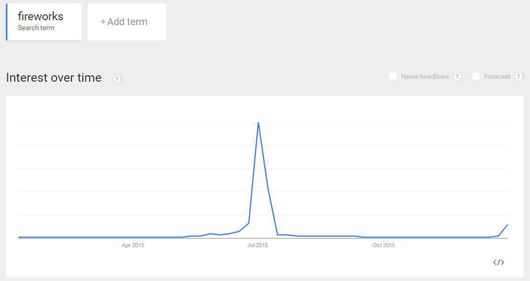
For example, in the U.S., Google searches for “fireworks” correlate positively with temperature throughout the year, but only because July 4th is in the summer. This is a seasonal effect, not a weather effect.
 Almost every weather paper tries to control for seasonality. This post shows they don't control enough.
How do they do it?
To answer this question, we gathered a sample of 10 articles that used weather as a predictor. [1]
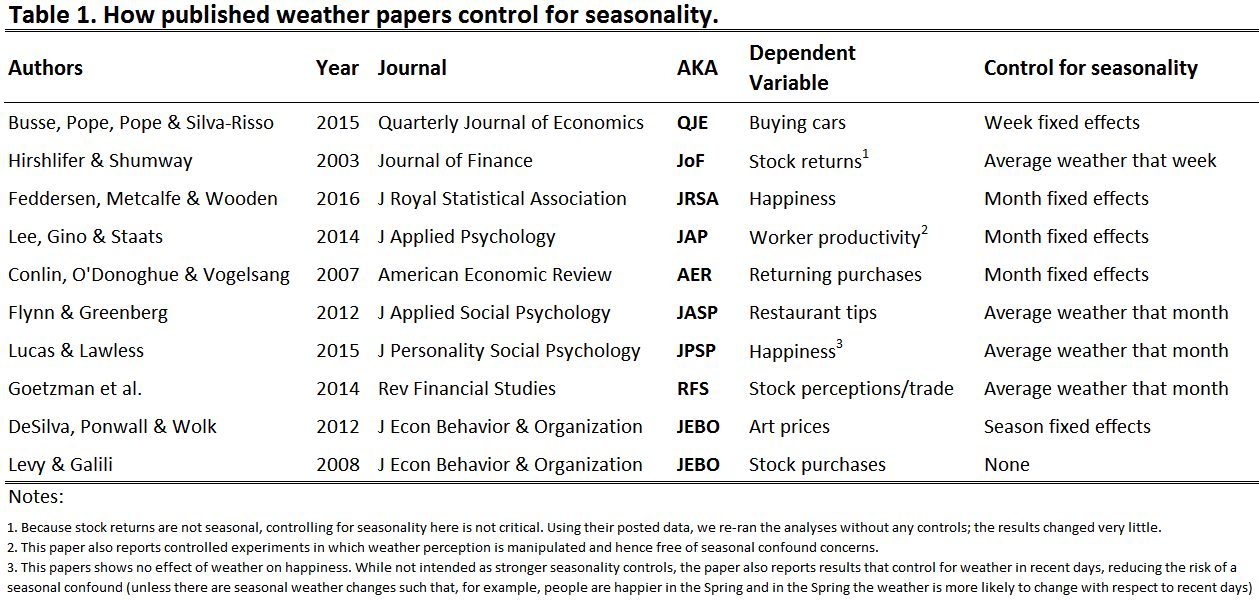 In economics, business, statistics, and psychology, authors use monthly and occasionally weekly controls to account for seasonality. For instance they ask, “Does how cold it was when a coat was bought predict if it was returned, controlling for the month of the year in which it was purchased?"
That’s not enough.
The figures below show the average daily temperature in Philadelphia, along with the estimates provided by monthly (left panel) and weekly (right panel) fixed effects. These figures remind us that the weather does not jump discretely from month to month or week to week. Rather, weather, like earth, moves continuously. This means that seasonal confounds, which are continuous, will survive discrete (monthly or weekly) controls.
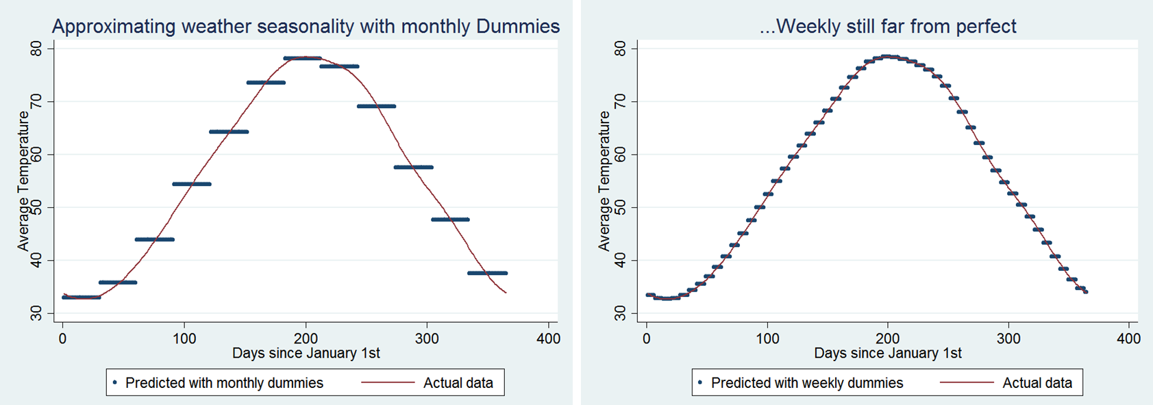 The vertical distance between the blue lines (monthly/weekly dummies) captures the residual seasonality confound. For example, during March (just left of the ‘100 day’ tick), the monthly dummy assigns 44 degrees to every March day, but temperature systematically fluctuates within March, from a long-term average of 39 degrees on March 1st to a long-term average of 50 degrees on March 31st. This is a seasonally confounded 11-degree difference that is entirely unaccounted for by monthly dummies.
The confounded effect of seasonality that survives weekly dummies is roughly 1/4 that size.
Fixing it.
The easy solution is to control for the historical average of the weather variable of interest for each calendar date.[2]
For example, when using how cold January 24, 2013 was to predict whether a coat bought that day was eventually returned, we include as a covariate the historical average temperature for January 24th (in that city).[3]
Demonstrating the easy fix
To demonstrate how well this works, we analyze a correlation that is entirely due to a seasonal confound: the number of daylight hours in Bangkok, Thailand (sunset – sunrise), and the temperature that same day in Philadelphia (data: .dta | .csv| ). Colder days in Philadelphia tend to be shorter days in Bangkok, but not because coldness in one place shortens the day in the other (nor vice versa), but because seasonal patterns influence both variables. Properly controlling for seasonality should eliminate an association between these variables.
Using day duration in Bangkok as the dependent variable and temperature in Philly as the predictor, we threw in monthly and then weekly dummies to control for the seasonal confound. Neither technique fully succeeded, as same-day temperature survived as a significant predictor. (STATA .do)
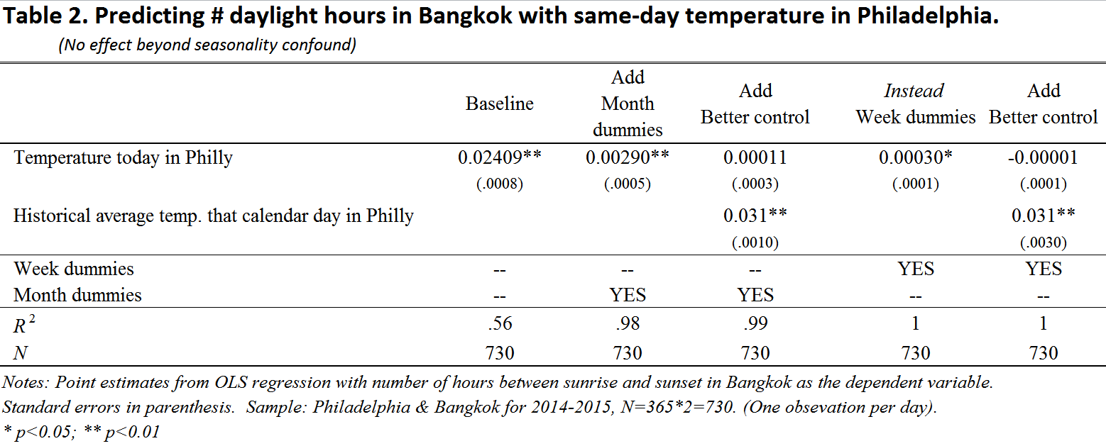 Thus, using monthly and weekly dummy variables made it seem like, over and above the effects of seasonality, colder days are more likely to be shorter. However, controlling for the historical average daily temperature showed, correctly, that seasonality is the sole driver of this relationship.
![]()
Original author feedback:
We shared a draft of this post with authors from all 10 papers from Table 1 and we heard back from 5 of them. Their feedback led to correcting errors in Table 1, changing the title of the post, and fixing the day-duration example (Table 2). Devin Pope, moreover, conducted our suggested analysis on his convertible purchases (QJE) paper and shared the results with us. The finding is robust to our suggested additional control. Devin thought it was valuable to highlight that while historic temperature average is a better control for weather-based seasonality, reducing bias, weekly/monthly dummies help with noise from other seasonal factors such as holidays. We agreed. Best practice, in our view, would be to include time dummies to the granularity permitted by the data to reduce noise, and to include the daily historic average to reduce the seasonal confound of weather variation.
Footnotes.
- Uri created the list by starting with the most well-cited observational weather paper he knew – Hirshlifer & Shumway – and then selected papers citing it in the Web-of-science and published in journals he recognized. [↩]
- Another is to use daily dummies. This option can easily be worse. It can lower statistical power by throwing away data. First, one can only apply daily fixed effects to data with at least two observations per calendar date. Second, this approach ignores historical weather data that precedes the dependent variable. For example, if using sales data from 2013-2015 in the analyses, the daily fixed effects force us to ignore weather data from any prior year. Lastly, it 'costs' 365 degrees-of-freedom (don’t forget leap year), instead of 1. [↩]
- Uri has two weather papers. They both use this approach to account for seasonality. [↩]