A few years ago our Journal Club discussed an interesting methods paper entitled, “Putting Psychology to the Test: Rethinking Model Evaluation Through Benchmarking and Prediction” (.htm). This post describes my attempt to understand what’s happening in Figure 1 of that paper, which shows that extremely simple experiments can generate extremely negative R2s. I learned a lot, much of it unexpected (at least to me) and interesting (at least to me). In this post, I’ll share what I learned [1]. The data and code for this post are here: https://researchbox.org/6202.
Before I show you the figure that perplexed me, some background is necessary.
The paper makes many points, one of which is that our standard statistical procedures – like running basic OLS regressions on our full datasets – often convey an extremely optimistic impression of how good our models are at predicting new observations.
To help make that case, the authors analyzed data from Many Labs, an effort by many different labs around the world to try to replicate some published findings in psychology (.htm). The figure that sparked this post focused on replications of a sunk cost effect, in which participants were randomly assigned to one of two conditions and then submitted a rating on a 9-point scale (the details aren’t critical, but if you want them they are here: [2]). Specifically, it plots the results from 15 labs that found a statistically significant effect of the manipulation on the dependent variable [3]. The models producing these results could not be simpler: regressing ratings on experimental condition (0 = control; 1 = treatment). That’s it. No additional variables.
The figure compares the R2 estimates that those labs obtained using OLS regression (orange dots) to the R2 estimates that these authors obtained using 10-fold cross validation (purple dots). It lists each of the 15 Many Labs sites on the y-axis and represents the R2s on the x-axis. Here it is, along with my annotations; the figure note is theirs:
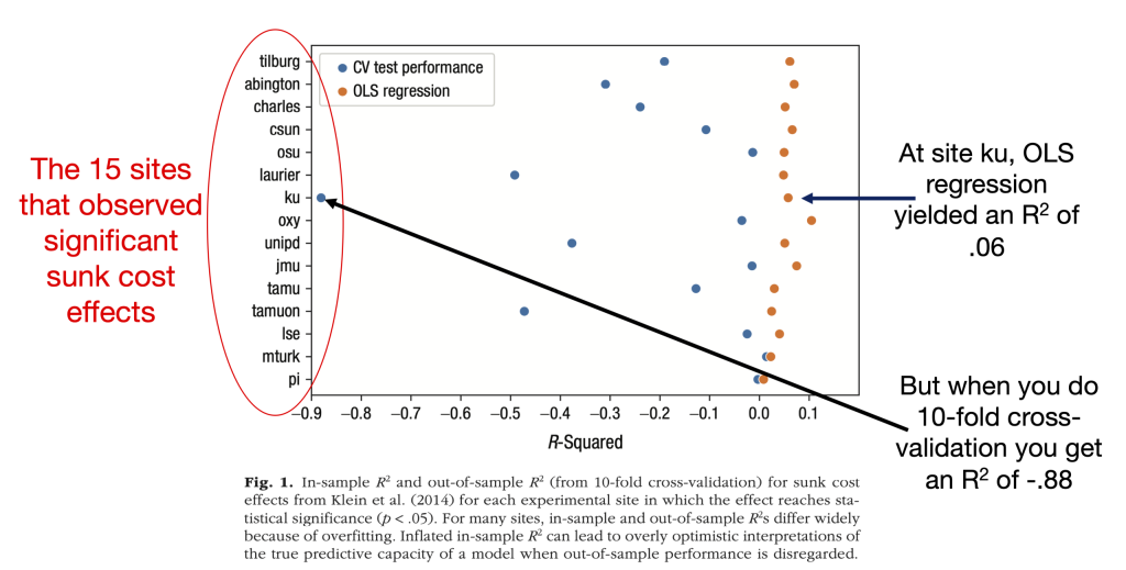
The takeaway is that the cross-validation estimates are always lower than the OLS estimates, and in many cases much lower. For example, the median OLS R2 is .051, and the median cross-validation R2 is -.128.
The authors interpret this as evidence that the “R2s differ widely because of overfitting” and that the OLS estimates are “overly optimistic.” But that is not obvious to me. I had at least two questions.
- Most of the cross-validation R2s are negative. Indeed, one of them – for the “ku” sample – is very negative. What??
- Overfitting happens when a model fits (in-sample) data in a way that does not generalize to other (out-of-sample) data. This problem is much more likely when models are complex, contorted to fit the data that it is analyzing. But this model is built on a single binary predictor, a situation in which overfitting seems almost impossible. What??
I am no expert on cross-validation, and I wanted to understand these things. To do so, I dug into the authors’ posted (and helpfully immaculate) code. But before I tell you what I found, there are two things you need to understand first: (1) What is 10-fold cross-validation? and (2) How can R2 be negative?
What is 10-fold cross-validation?
To perform cross-validation, you build a model on one subset of data – called the training sample – and then use it to predict data in a different subset – called the test sample.
To perform 10-fold cross-validation, you divide the sample into 10 equally sized subsamples called folds. So if your dataset has a total of 100 observations, you divide the sample into 10 folds of 10 observations each.
You then use Fold 1 as the test sample and build a model using the remaining 90% of the data (Folds 2-10). You use that model to predict the Fold 1 observations and measure how well it performs. You repeat this process nine more times, each time holding out a different fold as the test set.
The assessment of model performance can take many forms, but what the authors did was calculate an R2 for each fold – yielding 10 R2 values – and then average them. Those across-fold averages are what appear in Figure 1 [4].
How can R2 be negative?
Inconveniently, R2 means different things in different contexts.
For everyday OLS regressions, R2 represents the percentage of variance explained. And since you can’t explain negative percent of the variance, this R2 cannot be negative [5]. The authors refer to this as in-sample R2. I will refer to it as OLS R2 since it’s coming from our OLS regressions.
In the context of cross-validation, R2 is defined this way:
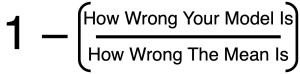
This cross-validation R2 is inherently comparative. It compares how well you’d do if you used your model to predict a set of values vs. how well you’d do if you simply predicted the mean every time. It is positive if your model does better than the mean, and negative if it does worse than the mean. In general, these R2 values can range from -∞ to +1 [6], [7].
Figuring Out Fold #9
In trying to understand Figure 1, I decided to focus on the outlier at the far left: the ‘ku’ sample’s (n = 113) very negative cross-validation R2 value of -.88. (‘Ku’ stands for Koç University in Istanbul. Go Rams.) I wanted to see exactly where that came from. So I ran the authors’ code, and I looked at the R2 values generated in each of the 10 folds. Here they are:
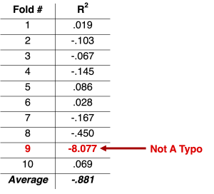
Check out Fold #9 and its gigantically negative R2 value of -8.077. Let’s see what’s going on there.
My first thought was that the model used to estimate the Fold #9 values must be a lot worse than the model used to estimate, say, the Fold #1 values. Let’s take a look at those models:
Fold #1 model: y = 6.66 + 1.15*treatment
Fold #9 model: y = 6.39 + 1.19*treatment
Um, those aren’t very different.
Fold #1’s model estimates a mean difference of +1.15, while Fold #9’s model estimates a nearly identical mean difference of +1.19. And yet the former has an R2 of .019 while the latter has an R2 of -8.077.
What??
To make sense of this, remember that these R2 values are comparative. They are comparing how well the model is doing against how well the mean is doing. This R2 value of -8.077 is not telling us that the model is doing terribly in an absolute sense. It is telling us is that it is doing terribly in a relative sense. The mean is doing a lot better at predicting the Fold #9 values than the model is.
To understand why, let’s take a look at the training sample data (n = 102) and test sample data (n = 11) used in Fold #9:
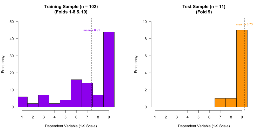
You can see that in the training sample, the values range from 1-9. But in the Fold #9 test sample, there is almost no variation. No values are below 7, most are equal to 9, and the mean is very close to 9.
This led me to ask a naïve question: When we compare the model’s performance to “the mean”, which mean are we using: the training sample mean (6.91) or the test sample mean (8.73)?
I was surprised to learn that in the land of cross-validation, the benchmark is the test-sample mean. That’s kinda brutal for the model, because the test-sample mean is a cheat: it is calculated from the very observations we are trying to predict. It effectively gets to peek at the answers.
By analogy, imagine I flip 10 coins, you predict 5 heads, but it turns out to be 7 heads. Your R2 will be negative, because although you (sensibly) predicted 50% heads, you had no chance against the observed mean of 70% heads. You’ll be punished for not foreseeing the unusual outcome.
You can’t beat the mean when every observation is equal to the mean.
That cross-validation R2 behaves this way is not a mistake. It’s simply how it is defined. It isn’t telling you that the model is generally bad or that the OLS R2 is extremely optimistic. It is telling you that, in this particular sample, a model built on 90% of the observations does worse than the observed mean at predicting the remaining 10% of observations. It is telling you something super specific, not something general about model performance.
Once you understand the machinery of all of this, you can see that, by the metric of R2, models stand very little chance when samples are really small. This is because small samples can be very unusual, containing observations that are unusually clustered, and thus very close to that sample’s mean. When I flip 10 coins, I might observe 70% heads. But when I flip 1,000 coins, I won’t. Similarly, when I observe 11-12 observations in the ‘ku’ sample, I might not see any values below 7, even though they range from 1-9 in the whole sample. But when I task the model with predicting a larger sample of observations, that happenstance clustering of values is less likely, the mean’s advantage shrinks, and the model has more of a fighting chance.
To illustrate this, what if instead of doing 10-fold cross-validation on the “ku” sample – which has us predicting folds containing 11-12 observations – we do 3-fold cross-validation – which has us predicting folds containing 33-34 observations? Note this is still an extremely small sample, and our model can still look bad. But we sure see a lot of improvement, with an R2 of .027 instead of -.881:
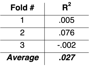
So making a small change to how cross-validation is done drastically changes the results.
Though I have focused on the small “ku” sample, it is worth noting that all but two of the 15 samples are small, containing fewer than 300 observations. Not coincidentally, the two large samples – mturk and pi – had cross-validation R2s that were pretty similar to the OLS R2s. But, in general, you can see that if we rebuild Figure 1 using 3-fold cross-validation, the R2s are better, and in fact mostly positive:
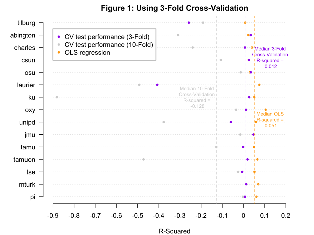
There is something peculiar about this. In 10-fold cross validation the models are built on 90% of the data, but in 3-fold cross-validation they are built on only 67% of the data. And yet, the models look better under 3-fold cross validation than under 10-fold cross-validation. That is, the models look better when you build them on smaller samples. This strange fact emerges entirely because R2 is comparative and the thing it compares against – the test-sample mean – has a bigger edge when the test samples are smaller (as in 10-fold cross-validation) than when they are larger (as in 3-fold cross-validation).
So the negative cross-validation R2s in Figure 1 don’t show that those OLS R2 estimates are wildly optimistic or that these simple models are somehow severely overfitting. Rather, they largely reflect how difficult it is for those models to outperform a structurally advantaged sample mean when test folds are very small.
So Are The Models Actually Overfitting?
R² can behave strangely in small samples. So instead of asking “how much variance is explained,” let’s ask a simpler question: how wrong are the predictions?
If a model is overfitting, it will be a lot worse at predicting new observations than at predicting the data it was trained on. For each of the 15 samples, we can use cross-validation to compare how far off the model’s predictions are when predicting new observations (out-of-sample error) vs. how far off they are when predicting the data it was trained on (in-sample error).
We can do this using two common performance metrics: Root Mean Squared Error – which gives greater weight to larger errors – and Mean Absolute Error – which simply represents the average mistake. The results are in the figure below. Note that the diagonal line marks the points at which the in-sample and out-of-sample errors are identical. Points above that line are consistent with overfitting (more error when predicting new observations than in-sample observations) and points below are consistent with underfitting (less error when predicting new observations):
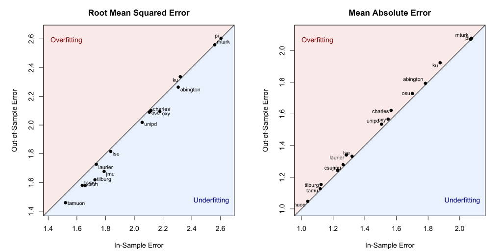
Across all 15 samples, those errors are nearly identical. In fact, the left panel shows that in 13 out of the 15 samples, the model made slightly smaller squared errors when predicting the new data than when predicting the data it was built on, more consistent with underfitting than with overfitting. The right panel shows slightly larger absolute errors in the out-of-sample than in the in-sample predictions, but the largest gap is only .06 points on this 9-point scale, hardly something to care about.
This evidence is much more consistent with the view that these simple models are not meaningfully overfitting than with the claim that they are.
Conclusion
In their paper, the authors make some important points. For example, in-sample R2 is generally optimistic about how well a model will perform on new data, behavioral scientists should care about how well our models forecast new observations, and we should adopt methods that allow us to evaluate that performance.
But that paper also included Figure 1, which, to a naïve reader like me, makes it look like even these simple models suffer from extreme overfitting; and that, if anything, those models are performing so poorly as to have no predictive value at all. That impression, I think, is misleading. Figure 1’s results look so dire because the authors are using R2 to assess cross-validated predictions in a context in which samples are very small. When you rely on different performance metrics – ones that don’t structurally disadvantage the model in very small test samples – you can see that these models are performing about as well as you’d expect given the modest effect sizes that the traditional analyses reveal.
From this post, you might take away some specific lessons about cross-validation or R2. But for me this exercise reinforced a broader lesson: Everything that scientists say hinges on the specifics of what they actually did. If you can’t (or don’t) evaluate the details, you can’t evaluate the science. I’m grateful to the authors for providing access to those details.
![]()
Author feedback
I shared an earlier draft of this post with the authors last summer, and they provided me with extremely helpful feedback that led me to significantly revise the post. I am very grateful for their feedback. I shared the updated draft with them more recently and they did not offer any additional feedback. If they do decide to comment or reply, I will post it here.
Footnotes.
- I make no claims that what I learned is new to the world; it was new to me, and so may be new to some of our readers.[↩]
- Participants imagined having tickets to see their favorite football team on a day on which it is freezing outside. They imagined that the tickets had been free or that they had paid for them, and they rated how likely they would be to go to the game, where 1 = definitely stay at home and 9 = definitely go to the game. Many Labs replicated the original finding: People rated themselves as more likely to go to the game when they paid for the tickets. (Across all labs the median cohen’s d was .31). Because people indicated being more likely to sit in the freezing cold if they had paid for the tickets than if they had gotten them for free, this is taken as evidence that people honor sunk costs.[↩]
- There were 36 labs in total, of which 15 found a significant effect. This post will focus only on those 15, since only those 15 results are contained in the figure.[↩]
- Really, you shouldn’t be averaging across them. You should be computing R2 by pooling over all predicted values. You don’t compute the standard deviation of a sample by chopping it into subsamples and averaging across those subsamples, because that’s not going to give you the same answer as computing the standard deviation of the whole sample. The authors did it this way because they used the sklearn package in Python, and that’s the way it does it. If you do the pooling instead of the averaging, Figure 1 looks a lot different: the lowest R2 is -.151 (instead of -.881) and the median R2 is -.031 (instead of -.128). The fact that this matters so much supports a thesis of this post – minor cross-validation decisions can severely influence the results – but going forward I’m going to ignore it.[↩]
- *Adjusted* R2s can be negative if the model is bad and there are many predictors that aren’t helping. We aren’t in that situation here – the models are significant and there is just one predictor – so we’ll ignore this.[↩]
- You get -∞ when all of the test observations are equal to the mean; in this case the mean perfectly predicts every value, and thus exhibits no error.[↩]
- Interestingly, and perhaps concerningly, when you use the most common cross-validation R package (caret), you never get negative R2s, because within each fold it computes the correlation between predicted and actual values and then squares it. So even if the predicted values negatively correlate with the actual values, the R2s will be positive. This means that you’ll get different answers if you use the most commonly used Python package vs. the most commonly used R package. Fun stuff.[↩]