When I taught my first PhD-level methods course, I invited students to submit questions about any topic in statistics or methodology. Six out of 10 students asked about the same topic: robust & clustered standard errors. It’s clearly a topic they found both important and confusing.
Psychologists basically never use robust standard errors.
But they always should. If you have never heard of robust SEs, this post is especially (rather than not) relevant for you.
Economists basically always use robust standard errors.
But I suspect intuitive understanding lags behind adoption. If you are robust SE user but don’t have an intuition for why robust errors can be (much) smaller than classical ones, this post is still relevant for you.
R Code to reproduce all figures https://researchbox.org/6145
Heteroskedasticity = “uneven noise”
Robust standard errors solve the problem of heteroskedasticity. This anglicized Greek compound word is an unnecessary mouthful. The underlying concept is straightforward: some data points are noisier than others. So, the noise in the data is uneven [1].
Noise, or sampling error, is simply how results would change if you had collected a different set of random observations (e.g., ask the same question of one random set of people vs. another).
Suppose we ask participants to guess the weight of a newborn vs. of this man on TikTok who uses the handle @thefatbutcher.

Disagreements about the newborn may be around 2 pounds, while those about the @fatbutcher could easily reach 20 pounds. This obvious fact produces uneven noise across data points: for the butcher vs. for the newborn. Which survey-respondent happens to answer our question about the butcher moves the data around by 20 pounds, while which survey-respondent happens to answer the question about the newborn by only 2 pounds.
The noise for the butcher is different from the noise for the newborn. Noise is uneven: heteroskedasticity.
More generally, observations with bigger values of the dependent variable will often have more noise than observations with smaller values. An extreme example is outliers: an observation that deviates from the rest by much more than expected is noisier than most observations [2].
Interestingly, ceiling and floor effects can produce the opposite pattern, more noise in the middle than the extremes. If we ask people to rate how wealthy someone is (1 = not at all; 10 = extremely), ratings of Bill Gates would get all 10s – no noise – while ratings of a truck driver’s wealth would get a wide variety of responses.

So this is what uneven noise (heteroskedasticity) is. Let’s now see why you should care.
From noise in the data to noise in the beta
Let’s imagine a regression predicting adult happiness with number of children.
The regression table could look something like this:
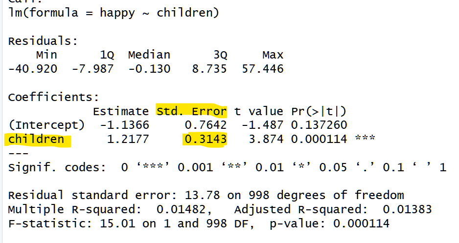
Source: entirely made-up data
The regression estimate says that happiness increases by 1.22 points per child.
We also have the standard error of that estimate: .31.
What does that standard error represent? It represents how much we expect the regression coefficient – the beta – to move around across new samples. Specifically, the standard error is the standard deviation of estimates across counterfactual samples. It is effectively a summary of how much noise is in the data, expressed in terms of how that noise in the data manifests as noise in the beta.
Let’s try to get an intuitive sense of how the regression computes the SE.
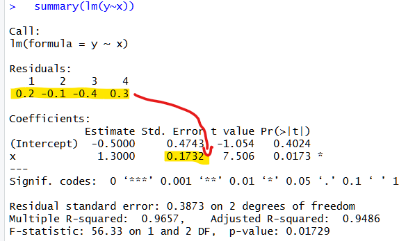
Let’s make super simple data:
x=1,2,3,4
y=1,2,3,5
Resulting in this simple plot:

The noise in the data is how far the dots are from the regression line, the residuals: .2, -.1, -.4, and .3.
A regression combines those four measures of noise in the data into the SE, a single number for the noise in the beta.
When you run a regression, lm(y~x), R uses math to go from 4 values to a single value.
The math does the equivalent of something like:
- Let’s imagine alternative datasets “like this one“, but with different noise
- Let’s run a regression in each of them and keep track of the beta
- The SE of our beta is the standard deviation of those other betas
One could do this with simulations, but the standard error is typically estimated with math (the math for standard errors is older than computer chips). The math makes assumptions about what datasets “like this one” may look like.
Most relevant to us today is the assumption of whether those datasets have
- Even Noise: all observations exhibit the same level of noise.
- Uneven Noise: some observations exhibit more noise than others.
If we assume all observations exhibit the same level of noise, all new imagined dots move by similar random amounts away from the regression line.
In our example above, the biggest data noise, 0.4, appeared when x = 3, but if we assume even noise, then we would assume that’s just a fluke. In the imagined datasets the noise = 0.4 would appear anywhere, in x=1, 2, 3, or 4. If instead we assume noise is uneven, new imagined datasets will tend to have the level of noise they had in the data we saw, so that the biggest error of 0.4 will once again tend to happen around x = 3, not around x=1, 2, or 4.
So why does this matter?
It matters because when going from noise in the data to noise in the beta it matters not just how much noise is in the data, but where the noise is.
Noise in the beta is more sensitive to noise in some datapoints than others.
When going from noise in the data to noise in the beta we don’t have a “one datapoint, one vote situation”.
The noise in some datapoints matters a lot, the noise in some datapoints is nearly irrelevant.
This is probably very far from obvious or intuitive, and I hope it is about to become both of those things.
Conference location
Say we have data on a bunch of researcher ratings of three candidate cities for a future conference: Caracas, Chicago, and Paris. We have the official tourism score for the three cities, 1, 50 and 100 respectively, and decide to run a regression to predict academic preferences with those tourism scores.

Source: totally made up tourism scores; the Caracas Lonely Planet cover is also made up.
Let’s say that on average academics’ preference for location is the same as the tourism score y = x, so 1, 50 and 100 for Caracas, Chicago & Paris respectively.
But academics don’t perfectly agree on anything, let alone conference location.
So not everyone gives those three scores; they only tend to do that on average.
Of interest to us today is noise, whether it is even or uneven across cities.
The figure below illustrates four stylized scenarios that will help you understand why where the noise occurs in the data matters for the noise in the beta.
 Fig 1. Even vs Uneven noise in data used for regressions
We start with the first box. Here we imagine that academics’ disagreement about locations has the same level across all three cities. The dots appear about as far away from the tourism score for all three cities.
Some academics think Caracas is much better than its tourism score, some much worse, and the same is true of all three cities. Even noise. Homoskedastic errors.
The next three boxes exhibit uneven noise. In box 2, the Chicago observations are the only highly variable option. Academics largely agree Caracas and Paris are as good as their tourism score, but disagree on Chicago. In the next two boxes, it is Paris and Caracas that academics disagree about.
Let’s consider how this noise will impact the other dataset we imagine. Let’s start with the first box, where the errors are even. Because there is noise all around, in one imaginary new dataset we could end up, just by chance, with more academics who like Caracas and dislike Paris, thereby flattening the line. Alternatively, we could also end up with academics who especially dislike Caracas and love Paris, steepening the line. So the line moves a fair amount across imagined datasets.
In the second box, in contrast, in new datasets Caracas is always around 1 and Paris always around 100. While Chicago jumps up and down, say between 65 and 35, it does not matter. Chicago noise is inconsequential. The straight line is always extremely similar. Moving on to the blue boxes, when the noise is in the extremes, the lines has much more noise than in the brown box, and also than in the green box.
An intuition for why the blue lines move more than the green line is that we take noise from the middle, where it does not matter, it does not impact the line, and we move it to the extremes, where it does matter.
The figure below illustrates this idea of the noise impacting alternative regression lines.
 Fig 2. How even vs uneven noise in data impacts regression lines across alternative datasets
Figure 2 is illustrative, showing regression lines I drew “by hand” to convey the intuition.
I did run actual simulations also, keeping track of the regression coefficient. The results are in Figure 3 below. We see that if the noise is even across the cities, the regression coefficient moves around less than if it is uneven and higher in the extreme, but moves more than if noise is uneven and concentrated in Chicago.
 Fig 3. Variability of regression coefficients, beta noise, when data noise is even vs uneven
Robust errors
Alright. So hopefully by now the following three things are intuitive:
- The standard error is a measure of noise in the beta
- Noise in the beta comes from noise in the data
- Which observations are noisy impacts how noisy is beta
Let’s now wrap it up with robust vs classical standard errors.
Classical standard errors, the ones taught in the first regression course, the ones that R prints when you run lm(y~x), assume noise is even, assuming every dataset is like the green box, whether they are, or whether they look like the brown or blue datasets. So even if all the noise is in one portion of the data, they assume that’s just a fluke, that the noise in other datasets could be anywhere.
Robust standard errors, in contrast, assume that other dataset will have the noise in roughly the same places as the observed data has it. If all the noise is in Caracas, it assumes other datasets will also have the noise in Caracas. Robust standard errors, therefore, give you different standard errors when the data are green, brown, or blue.
A stylized description that is very close to being literally true is that:
- Classical standard errors are the simple average noise, all residuals get equal weight
- Robust standard errors are a weighted average, residuals impacting beta more get more weight.
That weighted average, the robust SE, does a pretty good job.
In this last figure I plot the true variability of the regression coefficient across the 5000 simulations (the SD of the beta across simulations) and the different estimates next to it.

Fig 4. True and estimated standard error of regression coefficients with uneven noise
While it is obvious that classical errors can be quite terrible estimates, let’s point out the less obvious thing, which is that even if the data are homoskedastic, green bars, the robust errors do just as well as the classical ones. So you don’t need to worry about whether to choose classical or robust [3].
Robust errors is always the right call.
How to run robust standard errors?
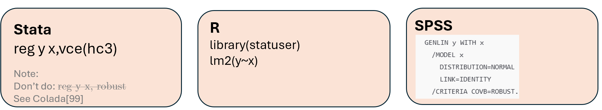
![]()
Footnotes.
- Technically speaking, lack of independence, which is addressed by clustered standard errors is also a heteroskedasticity problem[↩]
- Sometimes this is addressed by logging the DV, if the true function is not log(), however, there is still heteroskedasticity caused by specification error[↩]
- A reader of a draft of this post proposed that for small samples, in the absence of heteroskedasticity, classical errors can be smaller, so robust errors are not strictly superior. I ran simulations with a true linear model and homoskedasticity, n=100, R2=20%. The classical SE was smaller than the robust one in only 52% of simulations, and on average it was 0.06% (so 6 in 10,000) smaller. An absolutely ignorable downside of going robust[↩]