The authors of a forthcoming AER article (.pdf), “Methods Matter: P-Hacking and Publication Bias in Causal Analysis in Economics”, painstakingly harvested thousands of test results from 25 economics journals to answer an interesting question: Are studies that use some research designs more trustworthy than others?
In this post I will explain why I think their conclusion that experiments in economics are less p-hacked than are other research designs is unwarranted.
Disclaimer: I reviewed this paper for AER.
The authors conclude:[su_note note_color=”#e7f1f1″ radius=”1″]”our results suggest that the [instrumental variables] and, to a lesser extent, [difference-in-difference] research bodies have substantially more p-hacking and/or selective publication than those based on [randomized controlled trials] and [regression-discontinuity]” (p.3)[/su_note]
The authors base these conclusions on three main analyses:
[su_note note_color=”#e7f1f1″ radius=”1″]”We use three approaches to document the differences in p-hacking […]: [1] Test for discontinuities […] just above or below a conventional statistical threshold […] [2] [compare the […] proportion of tests that are marginally significant […] [3] comparing the observed distribution of test statistics […] to [the distribution] we expect to emerge absent p-hacking and publication bias.” (p.2&3)[/su_note]
In this post I will focus on approaches 1 & 2, which are basically the same for our purposes (approach 3 is discussed towards the end). Approaches 1 & 2 conclude there is more p-hacking when there are more results just below vs. above a significant cutoff (e.g., more p=.049s than p=.051s).
The figure below is a modified version of their Figure 2, showing histograms of collected z-values for two of the four literatures they review (recall, p=.05 when Z=1.96).
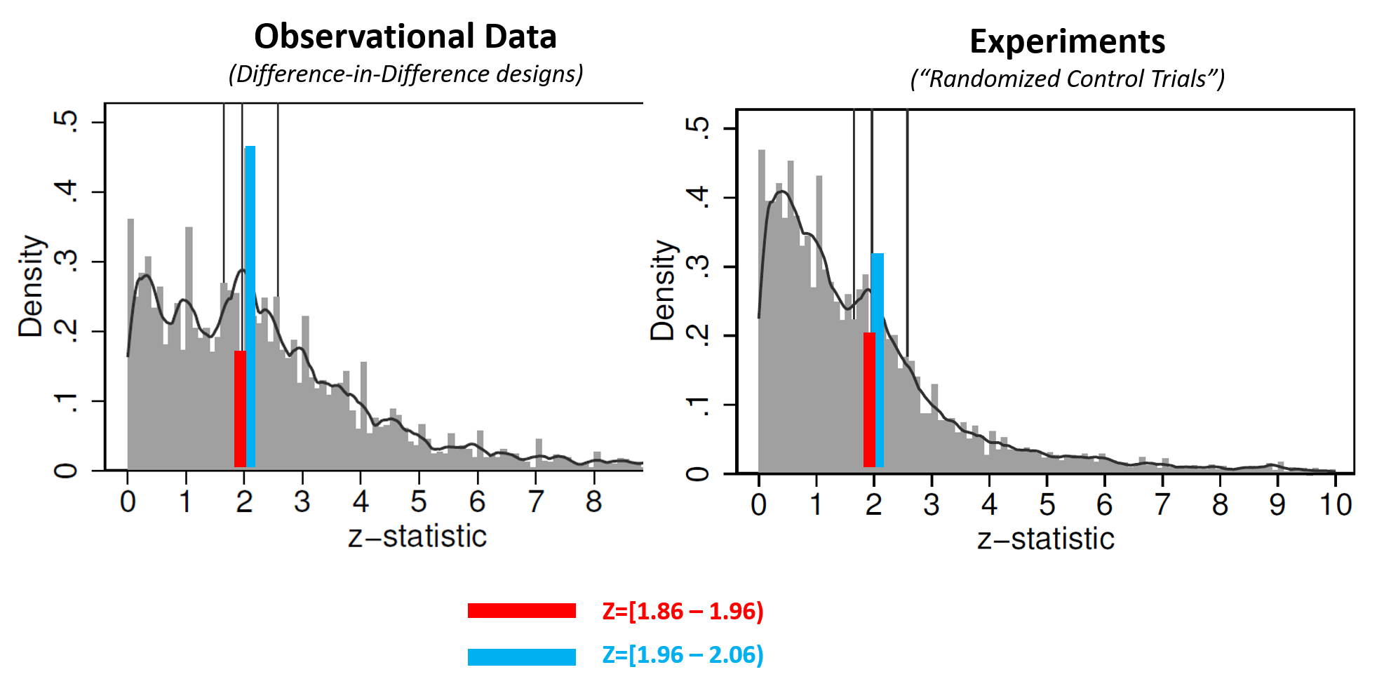
(For this post I added colored bars, panel titles, and the legend. See the original AER figure .png)
As the authors note, it is true that if there were no selective reporting, the red and blue bars should be about equally high. They are also right that the fact that those bars aren’t equally high implies that these literatures exhibit selective reporting.
It may be intuitively compelling to take one more logical step and assume the following: the more unequal the bars are, the more p-hacked a literature is. The authors rely on that assumption to conclude that experiments in economics are less p-hacked. But, the assumption is not correct.
Fast vs slow p-hacking.
Leif Nelson, Joe Simmons, and I coined the term p–hacking in our first p-curve paper (2014 | .htm). In Supplement 3 of that paper (.pdf), we modeled p-hacking as researchers computing, instead of just one p-value, a sequence of p-values. So researchers observe the p-value from the first attempted analysis, the p-value from the second attempted analysis, and so on. We used that framework to construct the expected distribution of p-values when a researcher engages in p-hacking. For this post all you need to know is that some forms of p-hacking change p-values more quickly than others.

Slow p-hacking arises when the p-value changes by a small amount from analysis to analysis. Say you run a regression with 25,000 observations and obtain p=.09. If you drop 57 observations and re-run the regression, the p-value will change, but probably by a small amount. You have basically the same data, run with the same statistical tool. When p-values change slowly, p-hacking will cause p-values to bunch below p=.05. The intuition is straightforward: if you approach p=.05 in baby steps, when you cross .05 you won’t land very far from it (≤ 1 baby step away). In studies with observational data, most available forms of p-hacking are probably slow: excluding a few observations here, transforming a variable there, expanding the before period by 2 weeks over there, etc. More generally, to analyze messy observational data we have to make lots of small operationalization decisions; most of these decisions will have small consequences on the final result, so p-hacking these decisions will usually constitute slow p-hacking. My intuition and non-systematic evidence suggest that slow p-hacking is more common in observational studies; but it is an unanswered empirical question.
Fast p-hacking arises when the p-value changes substantially from analysis to analysis. Say you run an experiment seeking to nudge people into vacuuming their couch more often. This is your one chance to run the couch-nudge study, so you include 14 manipulations (weekly vs. monthly reminders, opt-in/opt-out, gain/loss frames, etc.). The p-value comparing each pair of conditions will change substantially from pair to pair because the alternative tests are statistically independent. If one pair of conditions (say high vs. low sunk cost) obtained p=.72, another pair (e.g., vivid vs. dull images of couch-vacuuming) could easily be p=.001. Indeed, because p-hacking condition-pairs involves random draws from the uniform distribution (under the null), the p-value for two independent tests moves by 33 percentage points (from say p=.36 to p=.03, or vice versa) on average. My intuition and non-systematic evidence suggest that fast p-hacking is more common in experimental studies, especially costly field experiments; but it is an unanswered empirical question.
p-hacking fast and slow, a simulation.
To illustrate the association between fast vs. slow p-hacking and bunching below .05, I ran simulations where researchers use either slow p-hacking (highly correlated sequences of p-values, r=.75), or fast p-hacking (r=0). In both scenarios, p-hacking is equally consequential, increasing the false-positive rate from 5% to about 30%. Thus, both literatures are equally trustworthy (R Code).
For reasons explained earlier, p-hacking causes bunching only with slow p-hacking.
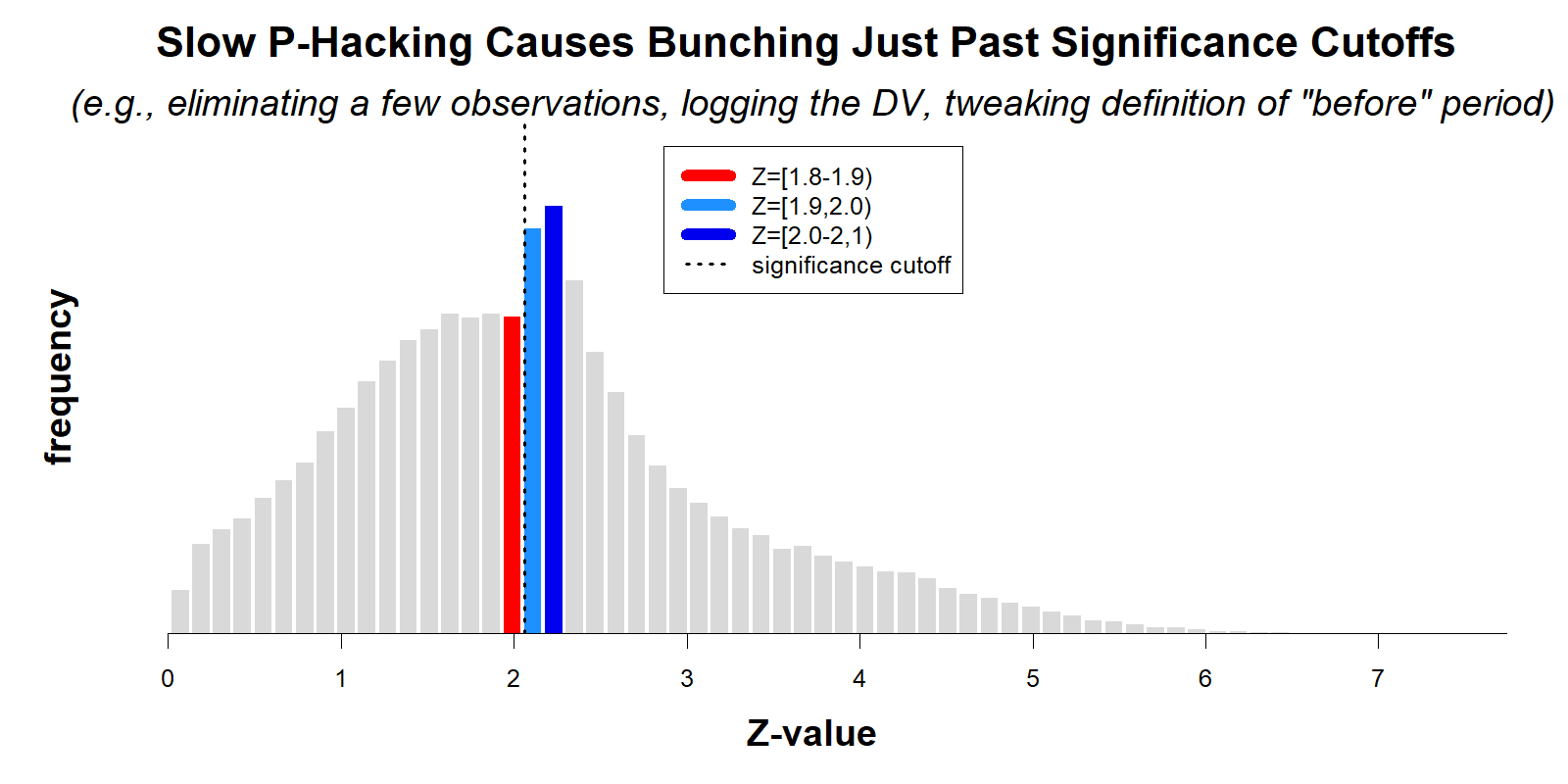
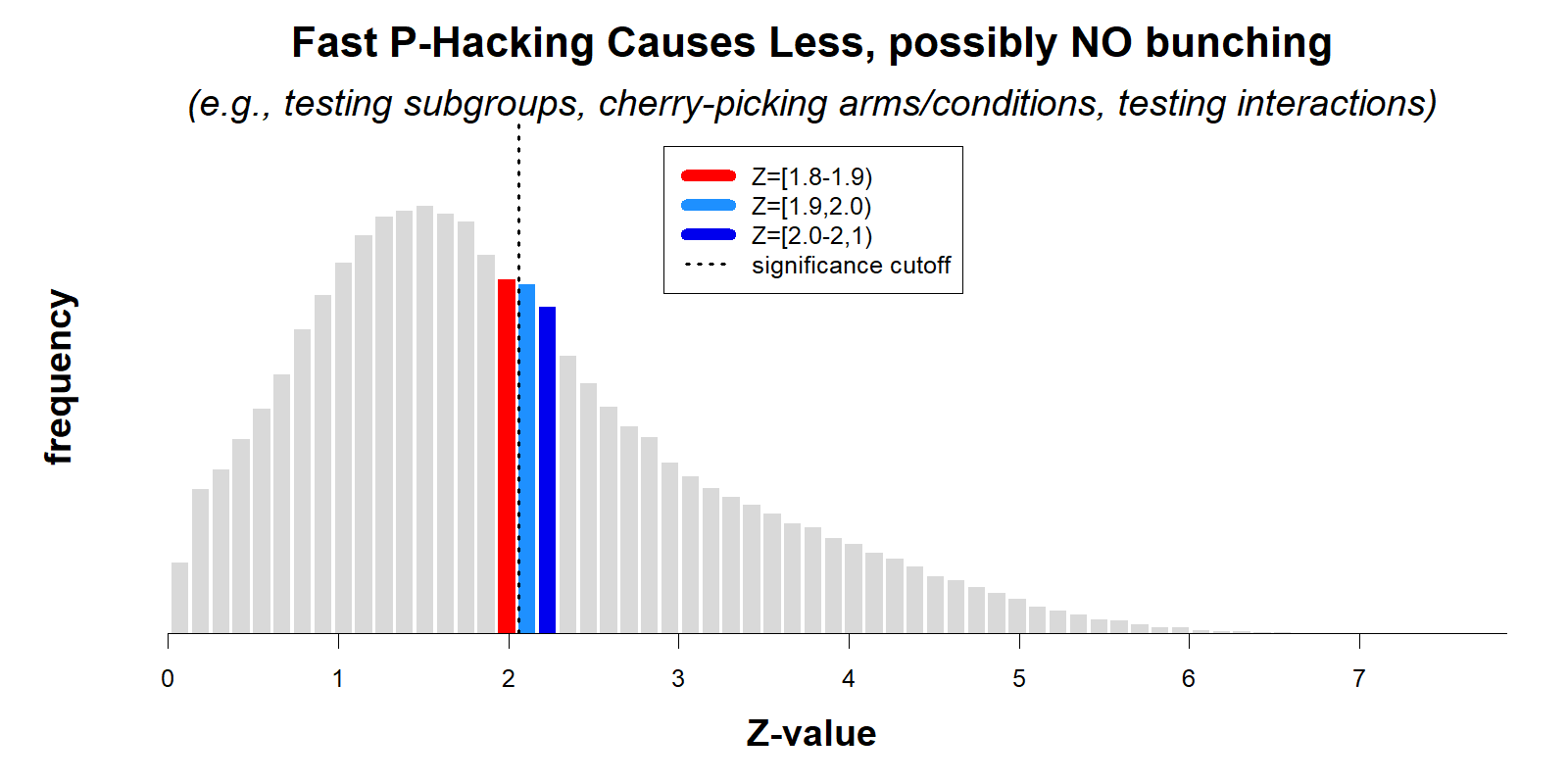 While both literatures have been p-hacked to the same extent (same consequences), the analyses from the AER paper would conclude the first literature is much more p-hacked and much less trustworthy than the second.
The third approach
So far I have focused on the first two approaches the AER paper used to assess p-hacking. The third method, recall, consisted of
[su_note note_color=”#e7f1f1″ radius=”2″]…[3] comparing the observed distribution of test statistics […] to [the distribution] we expect to emerge absent p-hacking and publication bias.” (p.3) [/su_note]
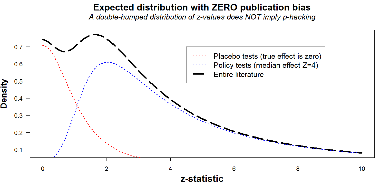
This comparison of expected and observed distributions leads to striking visualizations where publication bias is evident to the naked eye. For instance, the figure below is a slightly modified version of their results for the difference-in-differences literature. The ‘missing’ results below Z=2 really jump out.
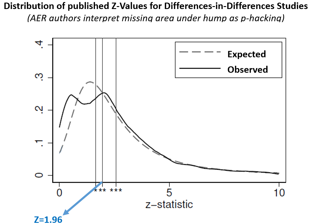
(modified version of the 1st panel in AER paper’s Figure 4 – see original .png)
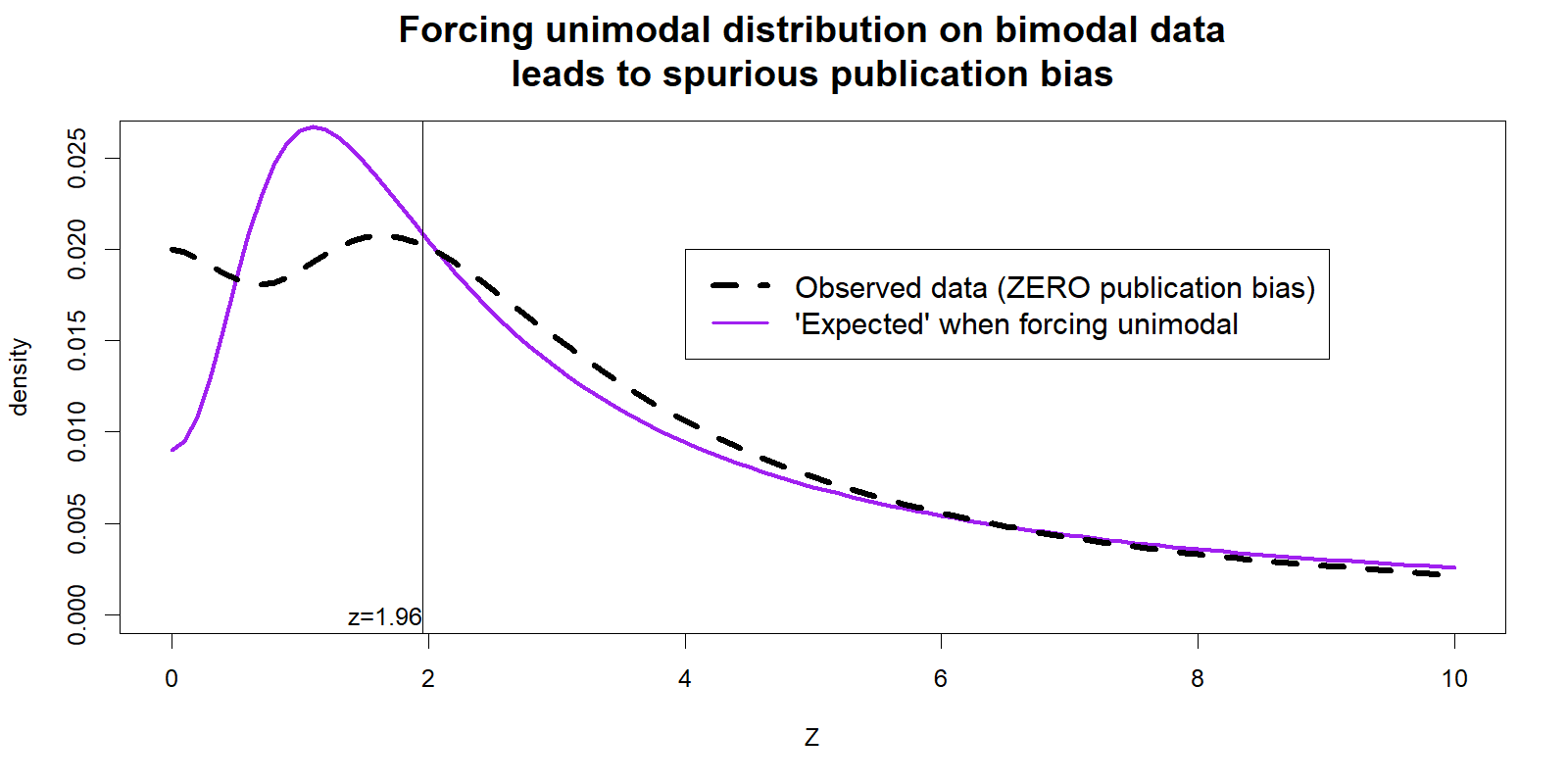
Unfortunately your naked eyes are deceiving you. This figure provides no evidence of publication bias because the ‘expected’ line is not really what we should expect.
Explaining this requires getting into the weeds, so you have to opt-in to read it.
Conclusion
I have proposed here that we should not infer that literatures with more bunching just past .05 are less trustworthy, and that visually striking comparisons of ‘expected’ and observed test results can be quite misleading due to incorrect assumptions about the expected line. Fortunately, there is a statistical tool designed exactly for the question this AER paper is interested on, where the evidential value of different literatures can be compared: p-curve.
P-curve has high power to detect evidential value and lack of it, it takes into account both slow and fast p-hacking, and it tells you not ‘whether’ there is selective reporting, but how strong the evidence for the effects of interest is once we control for selective reporting. I would not use p-curve, or any tool, however, to analyze 1000s of test results. The gains of a larger sample size become outweighed by the losses of interpretability and representativeness of any result.
You don’t need to know R to use p-curve, we made an online app for it: http://p-curve.com
![]()
Author feedback.
Our policy (.htm) is to share drafts of blog posts that discuss someone else’s work with them to solicit suggestions for things we should change prior to posting. About 2 weeks ago I shared a draft with the authors of the article who wrote a response which included some questions for me. You can read their revised full response here: [icon name=”file-pdf-o” class=”” unprefixed_class=””].pdf. Below I show the authors key comment/question in bold, followed by my comments.
1. Authors: How could slow vs fast p-hacking explain the differences in Instrumental Variables (IV) vs Regression Discontinuity Designs (RDD)?
Uri: I have read too few articles of each type to have a strong view, but my intuition is two fold. First, RDD hinges more strongly on ad-hoc operationalization decisions than does IV research, such as functional form assumptions and bin-size definitions. These decisions tend to have large consequences (fast p-hacking). But more importantly, and separate from the issues in this post, different research designs lead to reporting different sets of results, making comparisons of the distributions of all published test results across designs difficult to interpret. For example, say IV papers tend to report more robustness tests, while RDD papers tend to report more placebo tests. If both literatures had equal selective reporting, or equal evidential value, the set of all published results would have different distributions, different mixtures. The typical RDD paper in the AER sample had twice as many test results as the typical IV article did. To give a concrete example, an RDD article in the sample examined the impact of close elections on violence in Mexico and reported 8 (null) results for before the election. These are effectively placebo tests which should be, and are, near zero. (The RDD paper is doi:10.1257/aer.20121637, the 8 null findings from its Table 2 are in the AER dataset, see article id #46).
2. Authors: Should we really expect randomized control trials (RCT) to have more fast p-hacking?
Uri: The authors gave four arguments of why they don’t think that’s the case. (1) RCT are more collaborative (more ‘witnesses’), (2) are pre-registered, (3) reported to funders, and (4) difficult to just run and file-drawer whatever does not work. I think these are good arguments, and they gave me pause. I should make clear that I don’t know that RCTs have more fast, or slow, p-hacking than do other methods. I guess nobody does. There are reasons to expect more p-hacking in experiments, and there are reasons to expect less p-hacking. Precisely because we don’t know this, I object to relying on a statistical method that assumes we know this, and that we know it is identical across designs. To interpret bunching, we need to know how much fast and slow p-hacking happens. In addition, lots of p-hacking in the RCT literature is not hidden. Often RCT authors run many many tests, and report many tests, and then focus the discussion on the few significant ones. While transparent, this does not reduce the false-positive rate for the literature. (Some recent RCT studies control for some multiple comparisons.)
3. Authors: If we impose an assumption of a single round of fieldwork it would require that all the candidate nudges be tried at the same time, and the less favorable results then discarded. That seems to us a rather counterfactual to how RCTs actually work.
Uri: I got a bit into this in the previous point (at least some p-hacking in RCT is out in the open). In addition, I would say that: (1) manipulations are but one approach to fast p-hacking. Others include choosing subgroups (analyze just boys or just girls) and measures. I would also say (2) pre-registrations do not ‘prevent’ p-hacking but ‘simply’ make it easier to identify it. For this blue paragraph I just went to the SocialScienceRegistry (what some economists use for ‘pre-registration’), and searched for the name of a famous RCT researcher. Their first pre-registration to appear included the following eight variables as “primary” measures: “income, consumption, assets, nutrition, health, food security, financial behaviors, and labor supply.” Each, of course, is operationalizable in multiple ways, and many of them will be poorly correlated (fast p-hacking). In medicine, pre-registration has been required for clinical trials for years, and precisely thanks to those pre-registrations we know so many clinical trials are p-hacked (.htm).
The authors full response, again, is available here [icon name=”file-pdf-o” class=”” unprefixed_class=””].pdf
Footnotes.
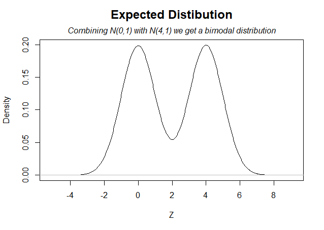
- I set ncp=2.78 for this second curve, inducing a median effect of about Z=4[↩]
- (To be clear, that the example generates a chart that resembles Figure 4 in the AER paper is not a coincidence. I chose the parameters to obtain that shape. In order to explain how one can obtain Figure 4 in the absence of publication bias, I need to produce Figure 4 without publication bias. We do not generally expect that particular shape in real literatures, there is no particular shape that can be generally expected. Part of the problem is precisely this, it is not possible to generate, based on statistical principles alone, the expected distribution of test results[↩]