[99] Hyping Fisher: The Most Cited 2019 QJE Paper Relied on an Outdated Stata Default to Conclude Regression p-values Are Inadequate

The paper titled "Channeling Fisher: Randomization Tests and the Statistical Insignificance of Seemingly Significant Experimental Results" (.htm) is currently the most cited 2019 article in the Quarterly Journal of Economics (372 Google cites). It delivers bad news to economists running experiments: their p-values are wrong. To get correct p-values, the article explains, they need to run, instead of regressions, something called "randomization tests" (I briefly describe randomization tests in the next subsection).  For example, the QJE article reads:

"[the results] show the clear advantages of randomization inference . . . [it] is superior to all other methods" (p.585). 

In this post I show that this conclusion only holds when relying on an unfortunate default setting in Stata. In contrast, when regression results are computed using the default setting in R [1], a setting that's also available in Stata, a setting shown over 20 years ago to be more appropriate than the one used by Stata (Long & Ervin 2000 .htm), the supposed superiority of the randomization test goes away.

Randomization is not superior, Stata's default is inferior.

In what follows I briefly explain randomization tests, then briefly explain the need for robust standard errors. Then I describe my re-analysis of the QJE paper.

All scripts and files for this post are available from https://researchbox.org/431 

Randomization Tests
Randomization tests are often attributed to Ronald Fisher, which is why the QJE paper's title begins with "Channeling Fisher", but this footnote explains why that may not be quite right [2].

Let's get a sense of how randomization tests work.

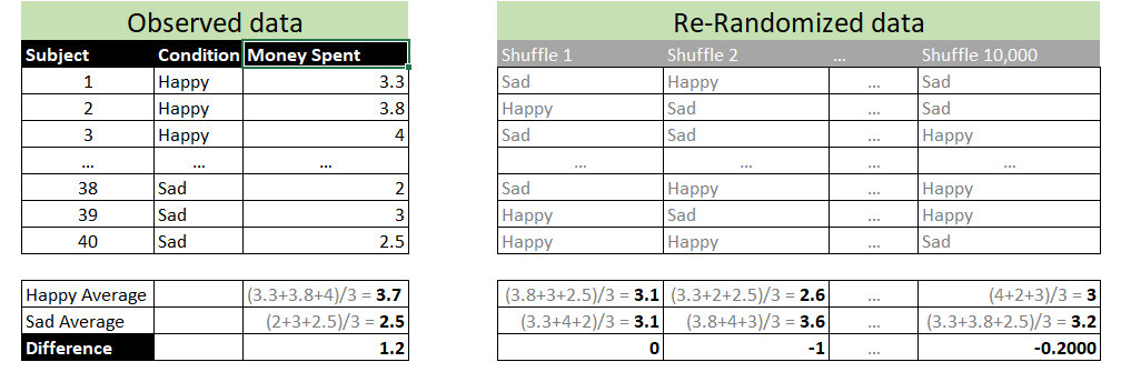
Say that in an experiment, participants are put in a happy vs sad mood and then they go shopping. Happy participants spend $1.20 more on average. To compute a p-value for this mean difference we could use a t-test, but we could also use a randomization test. For the latter, you randomly shuffle the condition column (Happy vs. Sad); see the gray columns in the table on the right above.  A datapoint from a participant in the happy condition can be re-labeled as sad, or stay happy, at random. You then compute the mean difference between the shuffled "happy" vs "sad" conditions. For example, the first shuffle leads "happy" and "sad" participants to, coincidentally, have means of $3.10, for a mean difference of $0.  You repeat this shuffling process, say, 10,000 times. You then ask: what % of the 10,000 shuffled datasets obtained a mean difference of $1.20 or more? That's your randomization test p-value [3].

Robust Standard Errors
Many readers know that "heteroskedasticity" describes something that can go wrong with a regression. In a nutshell, the problem is that the regression formulas assume that all observations are equally noisy, but in some situations some observations can be systematically noisier than others, creating a problem. To intuitively think of heteroskedasticity let's think about wine and academics.  When professors buy a bottle of wine, sometimes they spend a lot, and sometimes they spend little. When PhD students buy a bottle of wine, they always spend little. Professors' wine spending is thus systematically noisier than student wine spending. So wine spending is heteroskedastic. 

With heteroskedasticity, regression standard errors tend to be wrong, and thus p-values tend to be wrong.

The solution to incorrectly assuming all observations are equally noisy is to not assume that all observations are equally noisy, and to instead estimate how noisy each observation is. This is done by calculating robust standard errors, which are robust to heteroskedasticity.

Robust standard errors were developed surprisingly late in the history of statistics. White (1980) had the first major insight, and then MacKinnon & White (1985) developed what are today's most popular approaches to computing robust standard errors (See MacKinnon's (2013) review of the first 30 years of robust & clustered SE).

Note: the previous paragraph was added two weeks after this post was first published (also switching STATA->Stata). See the original version (.htm).

In any case, there are now five main ways to compute robust standard errors.
Stata has a default way, and it is not the best way.

In other words, when in Stata you run: reg y x, robust you are not actually getting the most robust results available. Instead, you are doing something we have known to be not quite good enough since the first George W Bush administration (the in-hindsight good old days).

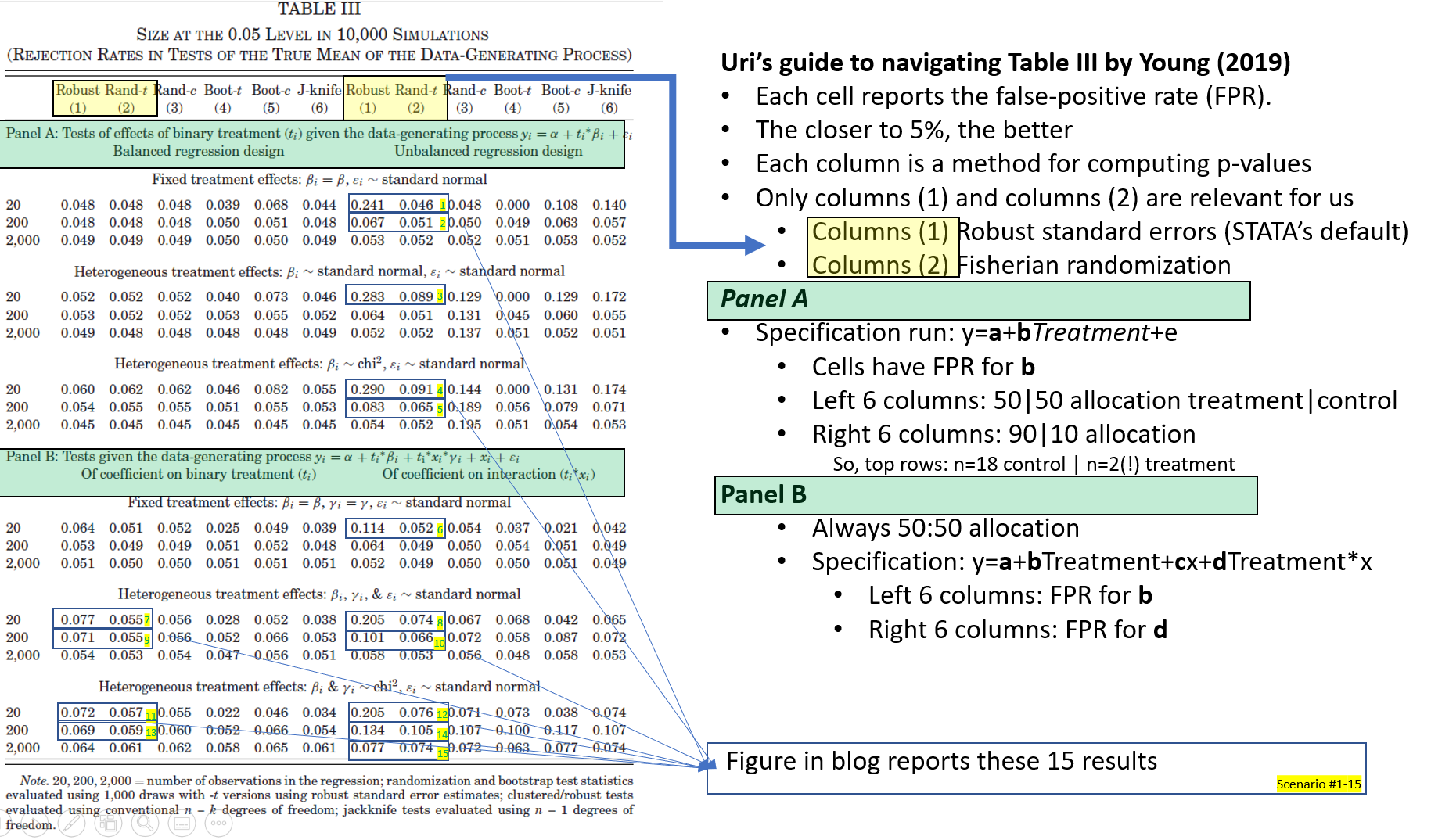
The five approaches for computing robust standard errors are unhelpfully referred to as HC0, HC1, HC2, HC3, and HC4.  Stata's default is HC1. That is the procedure the QJE article used to conclude regression results are inferior to randomization tests, but HC1 is known to perform poorly with 'small' samples. Long & Ervin 2000 unambiguously write "When N<250 . . .  HC3 should be used". A third of the simulations in the QJE paper have N=20, another third N=200.

So, the relevant question to ask during the (first) Biden administration is whether randomization is better than HC3 (Narrator: it is not).

Re-doing the simulations in the QJE paper
The QJE paper compares the performance of robust standard errors (HC1, i.e., Stata's default) with randomization tests for a variety of scenarios (involving various degrees of heteroskedasticity), by computing false-positive rates, that is, computing how often p<.05 is observed when the null is true [4]. The paper reports that regression results have false-positive rates that are too high, rejecting the null up to 21% of the time instead of the nominal 5%, while the randomization tests perform much better.

I think that the simulated scenarios in the QJE paper are too extremely heteroskedastic, making Stata's default look worse than it probably performs on real data, but I wanted to rely on the same scenarios to make it easy to compare my results with those in the QJE paper. Plus, I don't really know how much heteroskedasticity to expect in the real world.

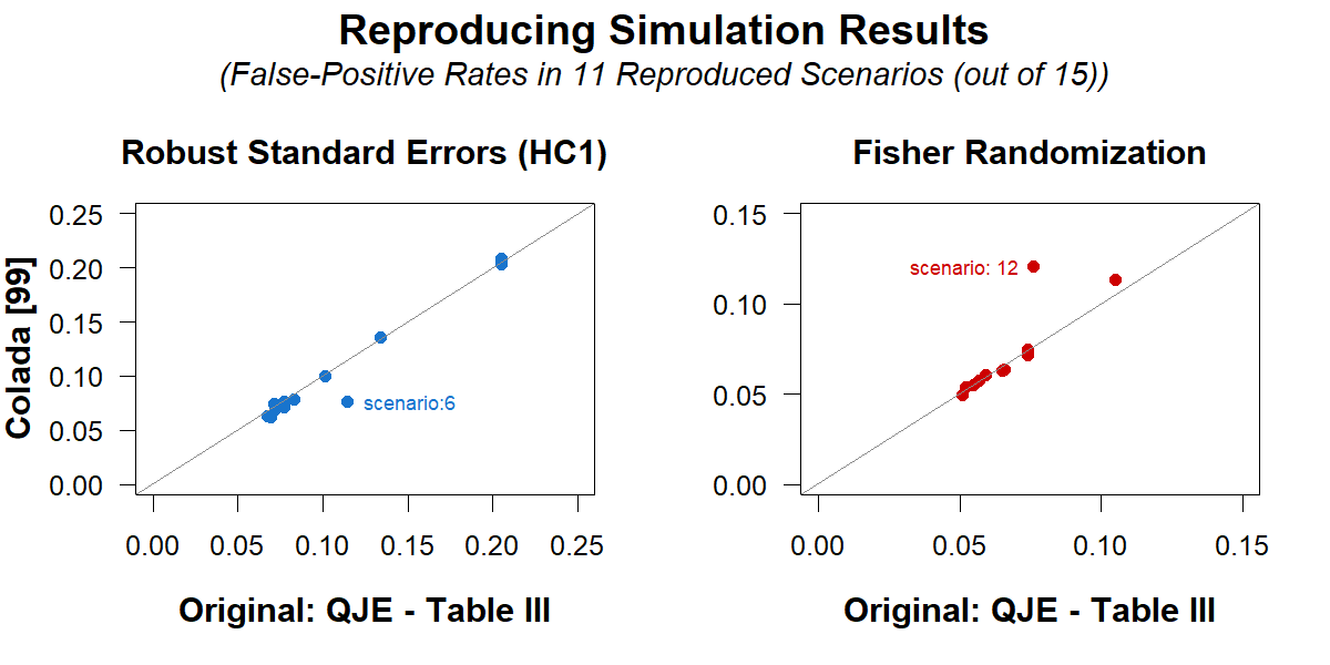
I began by successfully reproducing in R the reported simulation results (Table III of the QJE paper). Because I am focusing on the subset of scenarios for which regressions had an inflated false-positive rate (>6.5%), I made an annotated version of that Table III, that makes it clear which results I am reproducing. Most readers do not need to see it, but you can if you want Show Table III

After reproducing the published results, I re-ran the analyses using robuster standard errors (HC3).
All results are shown in the figure below [5].

The differences between blue and red bars reproduce the QJE results: Stata's default is worse than randomization.
The (mostly) lack of difference between the red and gray bars show that this is because Stata's default is especially bad, rather than because randomization tests are especially good. If anything, robuster standard errors outperform randomization tests in these scenarios.

This wraps up the point about randomization tests.

The QJE paper also re-analyzes data from 53 economics experiments and concludes "one of the central characteristics of my sample [of economics experiments] is its remarkable sensitivity to outliers" (p.566), adding "With the removal of just one observation, 35% of .01-significant reported results in the average paper can be rendered insignificant at that level." (p.567). I didn't have intuitions as to whether these numbers were actually troubling, so I looked into it. I don't think they are actually troubling. That proportion, 35%, is in the ballpark of what to expect when there are zero outliers. I wrote about this, but then after discovering the HC1 vs HC3 thing, worried it is too niche and makes the post too long, so I hid it behind the button below. 

I am curious about the outliers claim

Take home
I am a fan of randomization tests. They are useful when no accepted statistical test exists (e.g., to compare maxima instead of means), they are useful to run tests on complex data structures (e.g., we use it our Specification Curve paper .pdf to test jointly many alternative specifications run on the same data), they are useful for correcting for multiple comparisons with correlated data, they are useful for testing unusual null hypotheses (e.g., in fraud detection). But, if you are analyzing data with random assignment, in anything larger than a laughably small sample (n>5), why bother with a procedure that needs to be coded by hand (and is thus error prone), that is hard to adjust to complex designs (e.g., nested designs or stratified samples), and that does not deliver confidence intervals or other measures of precision around the estimates?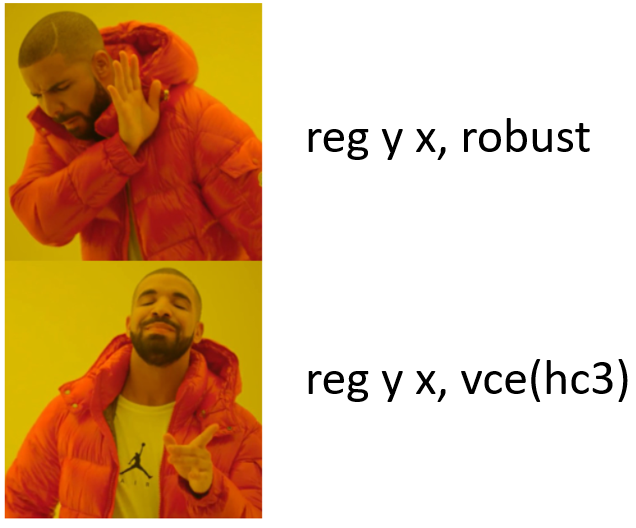

To produce digestible and correct empirical analyses we need to decide what is and what is not worth worrying about. For most papers, randomization tests are not worth the trouble.

But remember, when doing robust standard errors in Stata, either with experimental or non-experimental data:

Author feedback
Our policy (.htm) is to share drafts of blog posts that discuss someone else's work with them, to solicit suggestions for things we should change prior to posting, and to invite a response that is linked to from the end of the post (i.e., from here). I shared a draft of this post with Alwyn Young on September 30th, and then sent a reminder on October 9th, but he has not yet replied to either message. We did exchange a few emails prior to that, starting with an email I sent on September 9th, 2021, but that discussion did not involve the HC1 vs HC3 issue. I should probably point out that we have had n=99 blog posts so far, and removing a single observation, 100% of authors have replied to our emails requesting feedback.

References

• David, H. (2008 . htm) "The beginnings of randomization tests." The American Statistician 62.1 : 70-72.
• Long, J. S., & Ervin, L. H. (2000 .htm). Using heteroscedasticity consistent standard errors in the linear regression model. The American Statistician, 54(3), 217-224
• MacKinnon, J. G., & White, H. (1985 .htm). Some heteroskedasticity-consistent covariance matrix estimators with improved finite sample properties. Journal of econometrics, 29(3), 305-325. 
• MacKinnon, J. G. (2013 htm). Thirty years of heteroskedasticity-robust inference. In Recent advances and future directions in causality, prediction, and specification analysis (pp. 437-461). Springer, New York, NY.
• Simonsohn, U., Simmons, J. P., & Nelson, L. D. (2020 .htm). Specification curve analysis. Nature Human Behaviour, 4(11), 1208-1214.
• White, H. (1980 .htm). A heteroskedasticity-consistent covariance matrix estimator and a direct test for heteroskedasticity. Econometrica: journal of the Econometric Society, 817-838.
• Young, A. (2019 htm). Channeling Fisher: Randomization tests and the statistical insignificance of seemingly significant experimental results. The Quarterly Journal of Economics, 134(2), 557-598.

Footnotes.

1. Everything in R can be done in multiple ways; the default I am referring to is the one provided by the popular CRAN package sandwich .htm [↩]
2. A short article by David (2008 .htm) tells the history of randomization tests. Fisher discussed the idea only vaguely in his 1935 book, and Pitman, a statistician working in rather isolated Tasmania, developed randomization tests much more concretely in a 1937 article (.htm). This is subjective, but I think calling it Fisherian Randomization is an instance of the Matthew Effect (.htm). [↩]
3. Randomization tests are the modern incarnation of a permutation test, but instead of computing all possible permutations of the data (happy<-> sad), we compute a random subset of them. They are also a special case of a more general approach referred to as bootstrapping-under-the-null, which can be applied also to non-experimental data. For example, see the section "inference with non-experimental data" in our Specification Curve paper .htm [↩]
4. The QJE paper also reports results for 4 other approaches. They are more complicated and worse performing, so I do not discuss them here [↩]
5. In total I simulate 11 scenarios that are identical to scenarios in the QJE paper, so attempting to replicate 11 false-positive rates for Fisher randomization and 11 for robust standard errors (HC1). I obtain nearly identical estimates for 10 out of 11 of each set, but in each set I do obtain 1 substantially different result
   Show scatterplot comparing results

   
   One possibility for those large deviations is a copy-paste error into the paper's table in the originally reported results (the gaps are too large to be due to random simulation error). But I do not know the origin. The code for the QJE simulations is posted, but it is coded in Stata's MATA (.htm), a separate matrix programming language I am not familiar with. In addition, the 1500 lines of code are comments-free, except for section headers, so I was unable to chase this down discrepancy, which does not anyway alter the conclusions from this post.

   The scatterplot from this footnote, and associated calculations, are done in Section #7 in the R script available here: https://researchbox.org/431.13 [↩]