We typically ask if an effect exists. But sometimes we want to ask if it does not.
For example, how many of the “failed” replications in the recent reproducibility project published in Science (.pdf) suggest the absence of an effect?
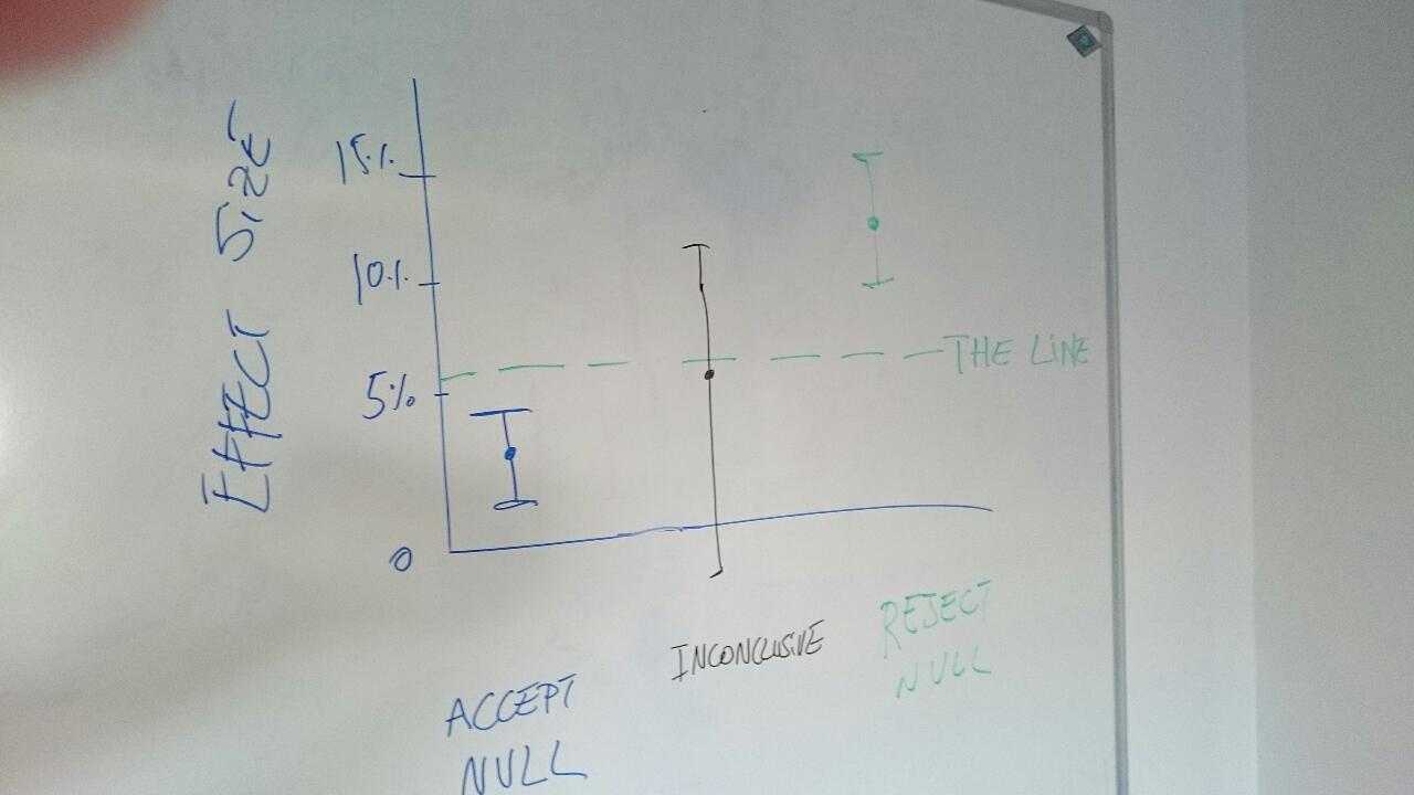
Data have noise, so we can never say ‘the effect is exactly zero.’ We can only say ‘the effect is basically zero.’ What we do is draw a line close to zero and if we are confident the effect is below the line, we accept the null.
 We can draw the line via Bayes or via p-values, it does not matter very much. The line is what really matters. How far from zero is it? What moves it up and down?
In this post I describe 4 ways to draw the line, and then pit the top-2 against each other.
Way 1. Absolutely small
The oldest approach draws the line based on absolute size. Say, diets leading to losing less than 2 pounds have an effect of basically zero. Economists do this often. For instance, a recent World Bank paper (.html) reads
“The impact of financial literacy on the average remittance frequency has a 95 percent confidence interval [−4.3%, +2.5%] …. We consider this a relatively precise zero effect, ruling out large positive or negative effects of training” (emphasis added)
(Dictionary note. Remittance: immigrants sending money home).
In much of behavioral science effects of any size can be of theoretical interest, and sample sizes are too small to obtain tight confidence intervals, making this approach unviable in principle and in practice [1].
Way 2. Undetectably Small
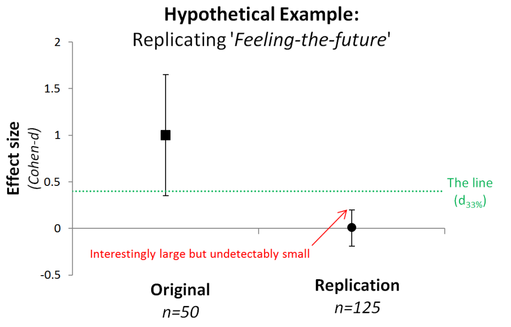
In our first p-curve paper with Joe and Leif (SSRN), and in my “Small Telescopes” paper on evaluating replications (.pdf), we draw the line based on detectability.
We don’t draw the line where we stop caring about effects.
We draw the line where we stop being able to detect them.
Say an original study with n=50 finds people can feel the future. A replication with n=125 ‘fails,’ getting and effect estimate of d=0.01, p=.94. Data are noisy, so the confidence interval goes all the way up to d=.2. That’s a respectably big feeling-the-future effect we are not ruling out. So we cannot say the effect is absolutely small.

The original study, with just n=50, however, is unable to detect that small an effect (it would have <18% power). So we accept the null, the null that the effect is either zero, or undetectably small by existing studies.
Way 3. Smaller than expected in general
Bayesian hypothesis testing runs a horse race between two hypotheses:
Hypothesis 1 (null): The effect is exactly zero.
Hypothesis 2 (alternative): The effect is one of those moderately sized ones [2].
When data clearly favor 1 more than 2, we accept the null. The bigger the effects Hypothesis 2 includes, the further from zero we draw the line, the more likely we accept the null [3].
The default Bayesian test, commonly used by Bayesian advocates in psychology, draws the line too far from zero (for my taste). Reasonably powered studies of moderately big effects wrongly accept the null of zero effect too often (see Colada[35]) [4].
Way 4. Smaller than expected this time
A new Bayesian approach to evaluate replications, by Verhagen and Wagenmakers (2014 .pdf), pits a different Hypothesis 2 against the null. Its Hypothesis 2 is what a Bayesian observer would predict for the replication after seeing the Original (with some assumed prior).
Similar to Way 3 the bigger the effect seen in the original is, the bigger the effect we expect in the replication, and hence the further from zero we draw the line. Importantly, here the line moves based on what we observed in the original, not (only) on what we arbitrarily choose to consider reasonable to expect. The approach is the handsome cousin of testing if effect size differs between original and replication.
Small Telescope vs Expected This Time (Way 2 vs Way 4)
I compared the conclusions both approaches arrive at when applied to the 100 replications from that Science paper. The results are similar but far from equal, r = .9 across all replications, and r = .72 among n.s. ones (R Code). Focusing on situations where the two lead to opposite conclusions is useful to understand each better [5],[6].
In Study 7 in the Science paper,
The Original estimated a monstrous d=2.14 with N=99 participants total.
The Replication estimated a small d=0.26, with a miniscule N=14.
The Small Telescopes approach is irked by the small sample of the replication. Its wide confidence interval includes effects as big as d =1.14, giving the original >99% power. We cannot rule out detectable effects, the replication is inconclusive.
The Bayesian observer, in contrast, draw a line quite far from zero after seeing the massive Original effect size. The line, indeed is at a remarkable d=.8. Replications with smaller effect size estimates, anything smaller than large, 'supports the null.' Because the replication is d=.26, it strongly supports the null.
A hypothetical scenario where they disagree in the opposite direction (R Code),
Original. N=40, d=.7
Replication. N=5000, d=.1
The Small Telescopes approach asks if the replication rejects an effect big enough to be detectable by the original. Yes. d=.1 cannot be studied with N=40. Null Accepted [7].
Interestingly, that small N=40 pushes the Bayesian in the opposite direction. An original with N=40 changes very little her beliefs about the effect, so d=.1 in the replication is not that surprising vs. the Original, but it is incompatible with d=0 given the large sample size, null rejected.
I find myself agreeing with the Small Telescopes' line more than any other. But that's a matter of taste, not fact.
![]()
Footnotes.
- e.g., we need n=1500 per cell to have a confidence interval entirely within d<.1 and d>-.1 [↩]
- The tests don’t formally assume the effects are moderately large, rather they assume distributions of effect size, say N(0,1). These distributions include tiny effects, even zero, but they also include very large effects, e.g., d>1 as probable possibilities. It is hard to have intuitions for what assuming a distribution entails. So for brevity and clarity I just say they assume the effect is moderately large. [↩]
- Bayesians don't accept and reject hypotheses, instead, the evidence supports one or another hypothesis. I will use the term accept anyway. [↩]
- This is fixable in principle, just define another alternative. If someone proposes a new Bayesian test, ask them “what line around zero is it drawing?” Even without understanding Bayesian statistics you can evaluate if you like the line the test generates or not. [↩]
- Alex Etz in a blogpost (.html) reported the Bayesian analysis of the 100 replications, I used some of his results here. [↩]
- These are the spearman correlation between the p-value testing the null that the original had at least 33% power, and Bayes Factor described above. [↩]
- Technically it is the upper end of the confidence interval we consider when evaluating the power of the original sample, it goes up to d=.14, I used d=.1 to keep things simpler [↩]
