In this post I show how one can analyze the frequency with which values get repeated within a dataset – what I call “number-bunching” – to statistically identify whether the data were likely tampered with. Unlike Benford’s law (.htm), and its generalizations, this approach examines the entire number at once, not only the first or last digit.
I first thought of this approach while I was re-analyzing data from the 2019 Psych Science paper on factory workers’ use of hand sanitizer (.htm) that Frank Yu, Leif Nelson and I discussed in DataColada[74]. In that post, we showed that the data underlying that paper exhibited two classic markers of data tampering: impossibly similar means and the uneven distribution of last digits (for numbers generated on a continuous scale). The authors issued a correction (.htm), and the editor expressed his concern (.htm).
After reading a draft of this second post, the first two authors of the article requested the paper be retracted, and that process is underway.
![]() Code to reproduce all figures and calculations in this post.
Code to reproduce all figures and calculations in this post.
Nudging hand-sanitizing
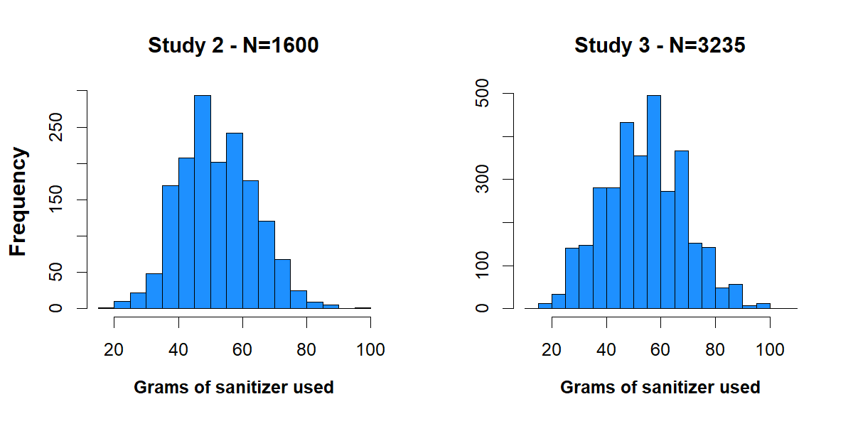
The Psych Science paper describes three experiments run in Chinese factories, where workers were nudged to use more hand-sanitizer. In this post I focus on Studies 2 and 3, where sanitizer use was measured to a 100th of a gram (for reference: a paper clip weighs about 1 gram). Let’s start with histograms of daily sanitizer use in the two studies:
Fig 1. Grams-Histograms in Studies 2 and 3
These histograms put many observations into each bin, so we don’t observe how often individual values are repeated. Figure 2 below zooms into Study 3’s histogram, giving an entire bin to each of the 8000 possible values between 20 and 100 grams.
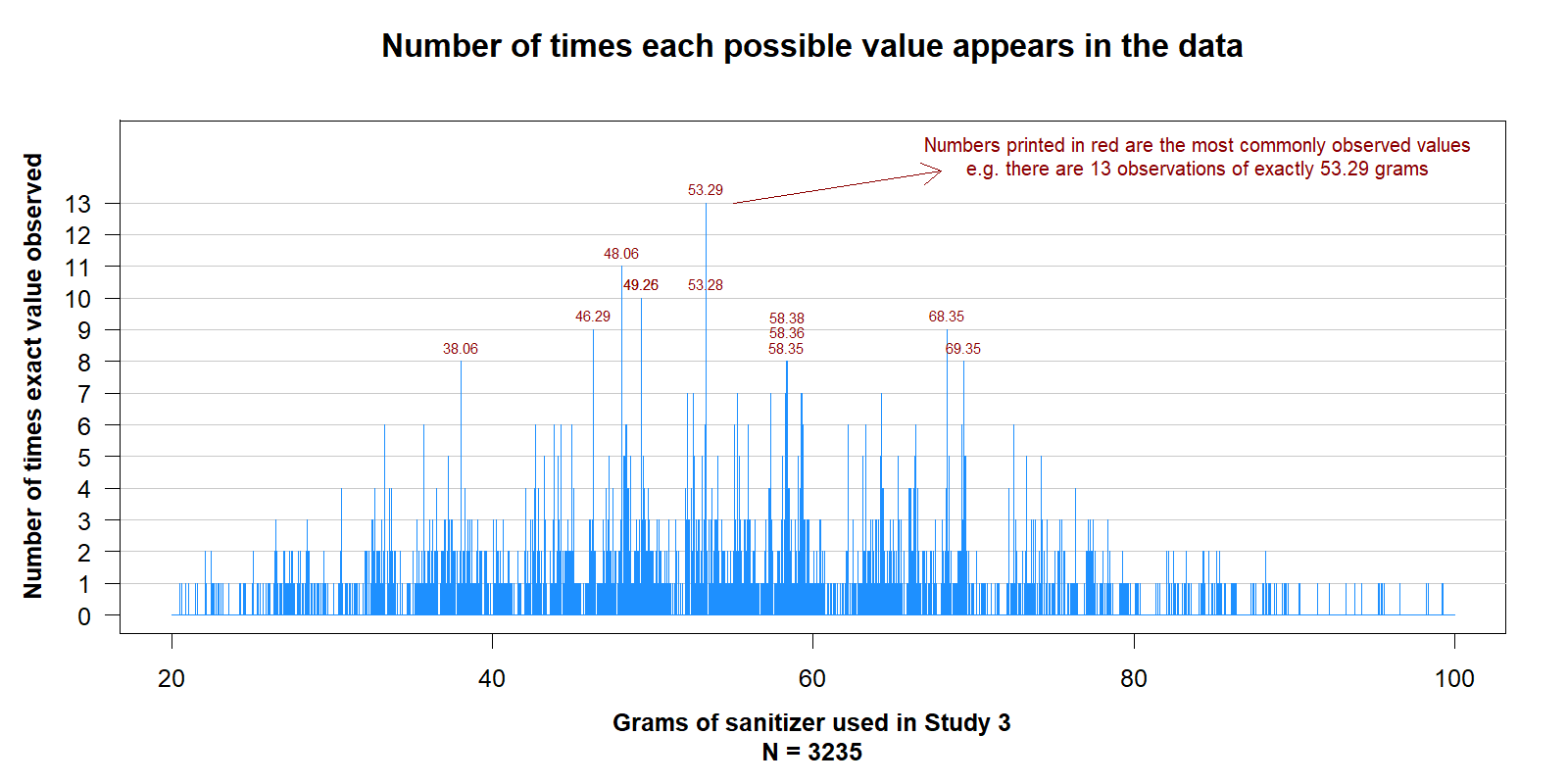 Fig 2. A fine grained histogram of Study 3. One bin per possible value.
Note: In the middle of the figure we see “58.38”, “58.36” and “58.35”, each of those three values appears exactly 8 times in the data.
The data seem intuitively bunchy. But how objectively surprising is Figure 2?
A p-value for number-bunching
To compute how extreme the observed level of bunching is, we need to (1) quantify bunching, and then (2) compare the observed level of bunching, to what would be expected if the data were not tampered with.
(1) Quantifying bunching
To quantify how bunchy the data are, I use the average-frequency of observed values. For example, if a dataset contained just 3 observations (11, 15, 15) the frequency of values for each datapoint would be (1, 2, 2) thus the average-frequency would be: (1+2+2)/3 = 1.67. Formula and details in this footnote [1].
(2) Expected-bunching
Because sanitizer use was measured to 1/100th of a gram, we can generate expected levels of number bunching by splitting gram values into an integer and decimal part, and then shuffling the decimal parts across observations. This effectively treats the decimal portion as random. This preserves the overall distribution of weights, as well as the exact frequency of every observed decimal value. All we are assuming here is that the (recorded) weight in grams is independent of its decimal portion (any observed number of grams could be associated with any observed fraction of grams). This test is thus independent of the already shown evidence that these data fail the uniform last digit test, for the (non-uniform) frequency of last-digits is maintained in the bootstrapped samples.
This is how the shuffling works:
 Fig. 3. Example of how decimals are shuffled to generate new data to compute expected level of bunching without making distributional assumptions.
We compute the average frequency for this shuffled distribution, repeat many times, and get a distribution of expected average frequencies, the expected level of number bunching. This approach is equivalent to a common way to bootstrap regressions, see footnote [2].
I will also report analogous calculations shuffling only the last digit of observed numbers. So, for example, 52.45 could become 52.48.
Results
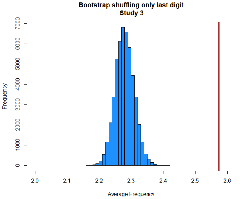
Figure 4 shows the expected average frequencies vs. the observed average frequency in the hand sanitizer use data. It is clear that the data contain many more repeated values than we would expect.
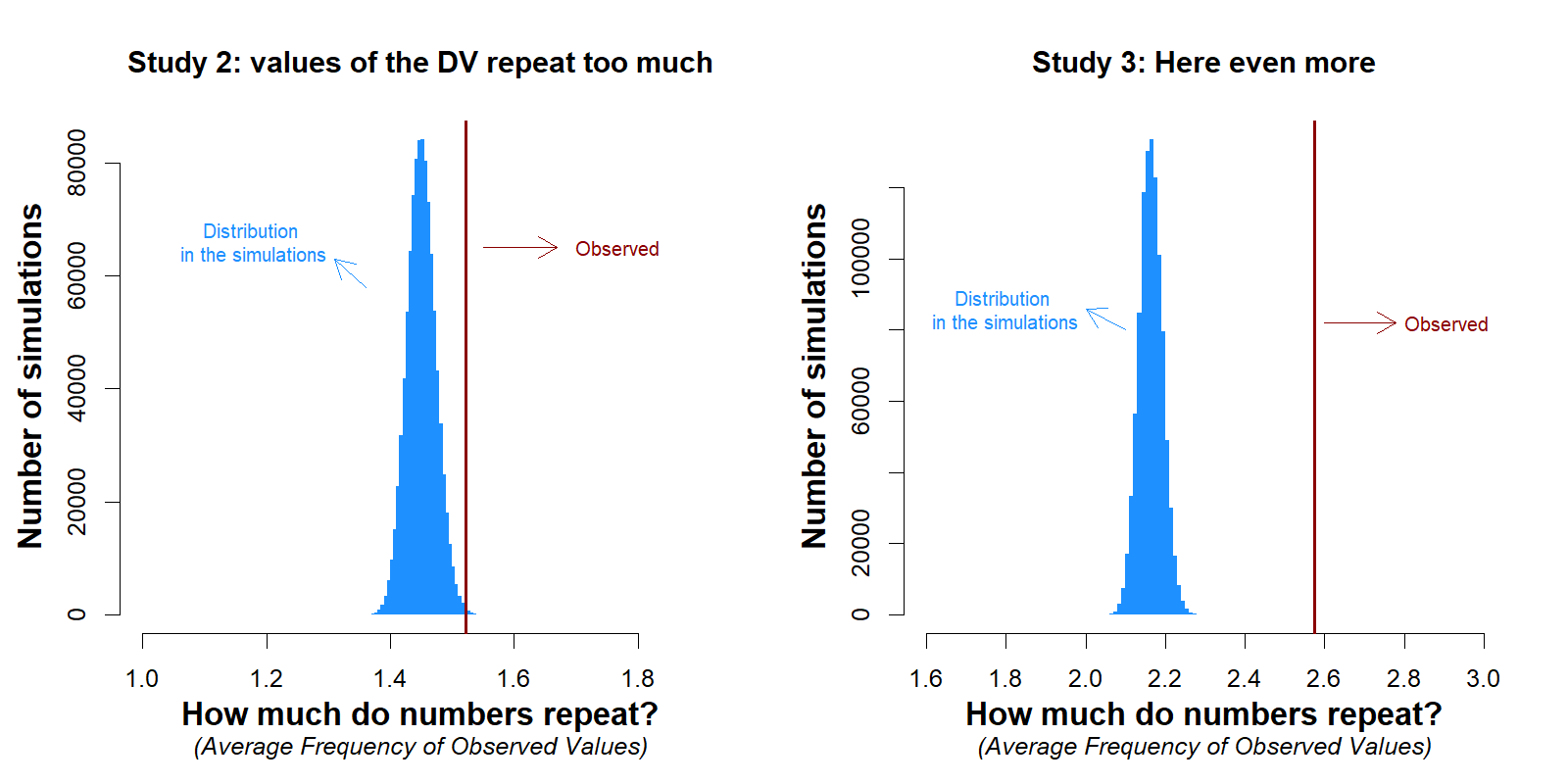 Fig 4. The data show more bunching than expected from real data.
In Study 2, we would expect the observed level of bunching to occur only 23 out of 10,000 times. In Study 3, we would expect the observed level of bunching to occur fewer than 1 in a million times.
If you perform the same analysis while shuffling only the last digit, instead of the last two digits, the results are essentially the same (figure in footnote [3] ).
Placebo tests
The number-bunching analysis used above, computing average frequency and shuffling decimals, is novel. It is important to apply it to some placebo datasets, expected be free of tampering. I applied it to two placebo datasets. The first comes from a study (.htm) weighting brood carcass mass with a scale also precise to 1/100th of a gram. The second dataset consists of a montecarlo simulation, generating data from the normal distribution matching the N, mean, and SD from Study 3. In neither case did the analysis suggest that these datasets contained too many repeated observations. [4].
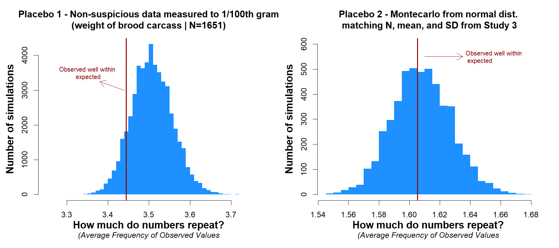
Fig 5. Number-bunching test does not flag placebos as suspicious
Possible explanations
This footnote explains why rounding (e.g., 44.99–>45.00) cannot explain the results [5].
Another possibility is that not all decimal values are equally likely with all integer values. For example, the scale may tend to report higher decimal values when the overall weight is lower. This footnote explains how I rule out that explanation [6].
Correlated decimals
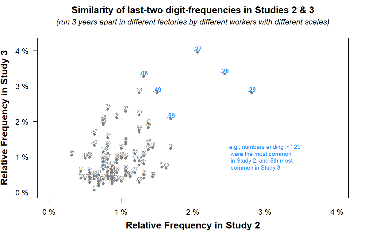
Evaluating the benign explanations discussed in the previous section lead me to find yet another anomaly present in these data: the frequency of decimal values is similar in Studies 2 and 3 (see Fig. 6).
Fig 6. Same decimal values are common in both studies. That should not happen.
For example, .27 was the single most common decimal value in Study 3, and it was the third most common in Study 2. The correlation of the frequency of decimal values across studies should be zero, but it is r = .54, p < 1/100 million. This implies a common source of ‘error’ for the anomalous number‑distributions in Studies 2 and 3.
That’s especially odd because Study 3 was run three years after Study 2, in a different factory, using a different scale, with sanitizer weighed by a different person(s).
Other uses of number-bunching anlaysis
Here I applied number-bunching analysis to a single sample (the entire study). I was able to do this because the data included an effectively random 1/100th of a gram level of precision. In general that's not the case (e.g., count data, likert scales, and willingness-to-pay data are not unnecessarily precise). In those situations we could use number bunching analysis when a null distribution is being considered. For example, we could test whether the last-two digits are distributed uniform in these data, using number bunching rather than a chi-square or a Kolmogorov-Smirnov test. For likely consequences of data tampering, the number-bunching approach has much more power. We can also use number-bunching analysis to make comparison across conditions. For example, are the data too evenly distributed across them? I hope to write about these extensions in a future post or paper.
![]()
Author feedback
Our policy (.htm) is to share drafts of blog posts that discuss someone else’s work with them to solicit suggestions for things we should change prior to posting. I shared a draft of this post two weeks ago with the first author of the hand-sanitizer paper and the editor of the journal. They provided a few suggestions to make the writing more neutral, which I welcomed and implemented. They also consulted with statistical experts and after such consultations they decided to retract the article.
- The formula for average-frequency, AF, is AF=sum(fi2)/sum(fi) where fi is the frequency of each distinct value i in the data. This metric is similar in spirit and formulation to entropy, which is commonly operationalized with entropy= – sum(pi*log(pi) ) where pi is the proportion of observation with each value (so pi=fi/N). But I prefer AF to entropy because it is a more intuitive metric, and generates interpretable values. For example, an average frequency of 2.5 means that, on average, observations contain a value that appears 2.5 times in the data, while an entropy of .68, say, is not an interpretable magnitude. In the simulations reported below, average frequency and entropy are highly correlated( |r| > .8). [↩]
- One approach to bootstrapping regressions consists of estimating a model, obtaining fitted values and the residuals from the estimated model, and then shuffling the residuals across observations. That's analogous to what's done here. If we used dummies for each integer value in the data as predictors, then the residuals would constitute the decimal portion of each number. The fitted value plus the shuffled residual would be the simulated data, as is the case here. [↩]
- Expected vs observed average-frequency when shuffling only the last digit of Study 3:
- For the montecarlo simulation, I plot one random draw here. I also run several thousand of them, verifying that the p-value from the bootstrap procedure was distributed uniformly across them. It was. [↩]
- A benign explanation for number bunching is that the scale used to weigh the sanitizer, or the human reading such scale, rounds values up or down, creating more identical values than would otherwise be expected. This would not be enough to explain the observed number-bunching, because the shuffling procedure keeps the share of rounded numbers the same (e.g., the share of .50s vs .49s). But it could account for it if rounding were more prevalent for some numbers. Say, 49.99 gets rounded to 50.00, but 27.99 does not get rounded to 28.00. But we can even rule out this possibility because Figure 2 shows that the most common numbers are not rounded (e.g., “53.29”). Also, if we leave rounded numbers out of the analyses altogether, the observed data is actually more surprisingly bunchy. [↩]
- There is a slight association, in Study 3, between the integer and the decimal value: the higher the integer, the lower the decimal value, r(integer,decimal)= -.12, p<.0001. This is yet another anomaly (with at least somewhat plausible benign explanations, not discussed here). In any case, within the range of values of 45 and 75 grams there is no association between the overall weight and the decimal value, r= -.01, p=.48, N=2,032. I thus repeated the shuffling procedure using only these data, asking if the observed average frequency of numbers in that range was too high as well. It was. The observed average-frequency (2.977) was 10 standard errors higher than what would have been expected by chance. The probability of this is less than 1 in a million. See Sections #6.4 and #6.5 in posted R Code [↩]

