[129] P-curve works in practice, but would it work if you dropped a piano on it?

P-curve is a statistical tool we developed about 15 years ago to help rule out selective reporting, be it p-hacking or file-drawering, as the sole explanation for a set of significant results. This post is about a forthcoming critique of p-curve in the statistics journal JASA (pdf).

The authors identify four p-curve properties they object to. Leaving aside some nuance, I agree that p-curve can exhibit those four undesirable properties. The disagreement is on whether they matter for practical purposes. (These four properties have long been recognized; see footnote for receipts [1])

The authors illustrate the four properties with carefully chosen edge cases. For example, in one such edge case they consider combining six p-values that are p < 1/750 trillion, with a seventh study that is p = 0.0499997. These edge cases are good for illustrating that something could possibly happen. These edge cases are less good for assessing whether something is likely to happen or to matter.

What I think is relevant but missing from the critique is any consideration of practical consequences, answering questions like:

How likely is p-curve to get it consequentially wrong?
Does any existing tool make fewer consequential errors?
If we abandoned p-curve, and went back to assuming there is no selective reporting, would inferences be better?

In this post I consider the practical implications of the two criticisms in the JASA paper that I thought may seem most persuasive to readers of the paper, or more realistically, to readers of shorter and more accessible renditions of the paper.

Criticism 1: p-curve’s results can get weaker when when including a stronger study (violating monotonicity).
Criticism 2: p-curve is overly sensitive to p-values extremely close to the cutoff (e.g., p = .05).

In an appendix I discuss the other two criticisms:
Criticism 3: heterogeneity biases p-curve's power estimator
Criticism 4: p-curve relies on the Stouffer method, which is "inadmissible"
("inadmissible" is a technical term that doesn't mean what you would expect it to mean).

Presenting p-curve's performance for implausible edge case, without considering performance under likely cases, is like testing cars by dropping pianos on them. The results would be spectacular and entertaining for some to watch. But, if a car failed the piano test it wouldn’t (and shouldn’t) influence car-buying decisions, because pianos are so unlikely to fall on cars.

Cars with objectionable performance in four imaginable piano-dropping tests

Criticism 1: Monotonicity Violations
P-curve only includes results that obtain p < .05. And for some analyses, only results that obtain p < .025.

The use of these cutoffs leads to a potentially undesirable property: it is possible for p-curve to violate monotonicity, a situation in which stronger study results produce a weaker p-curve summary.

I suspect that most p-curve users have come across this issue. You find a study with a strange hypothesis, a surprising analytical decision, and the critical result is p=.054. Because it is not p<.05, you cannot include it in p-curve. If the p-value had been a bit lower, if the analysts had tried an even more innovative analysis and gotten p=.049, you would include the result, and it would weaken p-curve. This violates monotonicity because a stronger p-value (p=.049 instead of p=.054) weakens p-curve's summary.

So that's the JASA paper's first concern.
I will propose this is not a big deal in practice in two ways.

First, I will tell you about other widely used tools that can also violate monotonicity.
Second, I will propose that p-curve is generally expected to be monotonic.

Popular statistical procedures that also can violate monotonicity
Example 1. Outlier exclusions
It is common to exclude outliers (e.g., observations that are 2.5 SD away from the mean), even though outlier exclusions violate monotonicity in the same way p-curve does. An observation that is 2.49 SD above the mean raises the mean, but one that is 2.51 SDs above the mean is excluded and so it does not. The most recent issue of Psychological Methods has a (Bayesian) paper (htm) relying on this monotonicity-violating procedure.

Example 2. Mixed-Models with random slopes
Consider a psychology experiment with 10 stimuli (e.g., 10 different disgusting sounds used to induce disgust). The data are analyzed with a mixed model that averages the overall effect across all stimuli. If one stimulus produces an effect much stronger than the others, its inclusion could weaken the overall summary—for instance, the analysis might yield p < .05 without that stronger stimulus, but p > .05 with it.

See footnote for intuition and R Code with example [2].

P-curve is expected to be monotonic
It is tricky to assess how likely or consequential monotonicity violations are, because they never really happen. Monotonicity violations involve counterfactual results. How would p-curve results have changed, if the studies in it became stronger? You can generate hypothetical counterfactual edge cases where this is a big deal, the JASA paper does, but those edge cases may not represent situations that are likely to ever happen, so they are not useful for making practical decisions.

I tried to run simulations that would answer the question: in general, should we expect p-curve to exhibit monotonicity. I did this in 5 steps:

Simulate 10 studies that are all powered at some level (e.g., 50%) [3].
Analyze those studies with p-curve.
Make all 10 p-values a tiny-bit stronger (I lowered them all by .001).
Analyze those modified studies with p-curve.
Compare 2 and 4. Did p-curve get stronger or weaker?

The results are in the figure below.

Figure 1. p-curve is generally expected to be monotonic
R Code to reproduce figure

Let’s start with the blue line, the results of the unmodified p-values. We see general monotonicity: The higher the true power of the underlying studies, the higher the power of p-curve. Stronger inputs, stronger outputs. Good.

Next, let's look at the red line, which shows the results of the modified p-values. The red line shows monotonicity in two ways: (1) it's also upward sloping (and thus monotonic), and (2) it's above the blue line. When p-values drop by .001, p-curve's power goes up.

That second result, 'red-line above blue-line' aggregates across all simulations. But I also kept track of whether each simulation violated monotonicity after reducing the p-values by .001. Those results are shown in the bottom of the figure: We see that it happened in between 0.2% and 2.8% of simulations. While monotonicity violations are possible, p-curve is more likely to move in the right direction: that's why the red line is above the blue line. Therefore, in expectation, p-curve is monotonic.

Criticism 2: p-curve is overly sensitive to p-values that are extremely close to the cutoff (e.g., p = .05)
The JASA authors point out that a p-value very close to the .05 cutoff (or the .025 cutoff) could have a disproportionate impact on the summary assessment, so that a bunch of very significant p-values can be annulled by one p-value very close to the cutoff.

We are totally on board with being concerned about outliers, so on board that we anticipated and addressed this problem in 2015 when designing the p-curve app. Specifically, the app reports how results change when you exclude its most extreme p-values. Unfortunately, the JASA paper did not mention the robustness tests our app generates.

Like the first criticism I will tackle this one in two ways.

First, I will assess how likely it is for a p-value very close to .05 to individually revert p-curve’s conclusions. Answer: unlikely.

Second, I will focus on those unlikely cases and ask: Does p-curve's diagnostic tool do a good job diagnosing this problem when it happens? Answer: yes.

Simulations on the impact of p-values close to .05
I ran simulations similar to those from the previous section: P-curves with 10 studies with power ranging from 35% to 80%. But now, instead of making those 10 p-values .001 smaller, I kept them as is and added an 11^th p-value that was very close to .05 (p=.04988) [4] .

That's an extremely high p-value. A study with 35% power has about a 1 in 2500 chance of obtaining a p-value between .04988 and .05, and the probability is lower for higher power. OK, so let's now see what this extremely high p-value would do if it showed up in a p-curve. The figure below shows a modest but sometimes non-trivial drop of power, between 0.1% and 5%.

Figure 2. The impact of adding a p-value extremely close to the cutoff (p = .04988)
R Code to reproduce figure

OK. Let's now consider an unlucky p-curver who finds themselves in this unlikely situation, would the p-curve app alert them to the problem? To make the case that the answer is yes, I submitted to the p-curve app one of those unlikely simulations in which the outlier p-value did change p-curve's conclusion.

Below is the relevant diagnostic plot from the app.

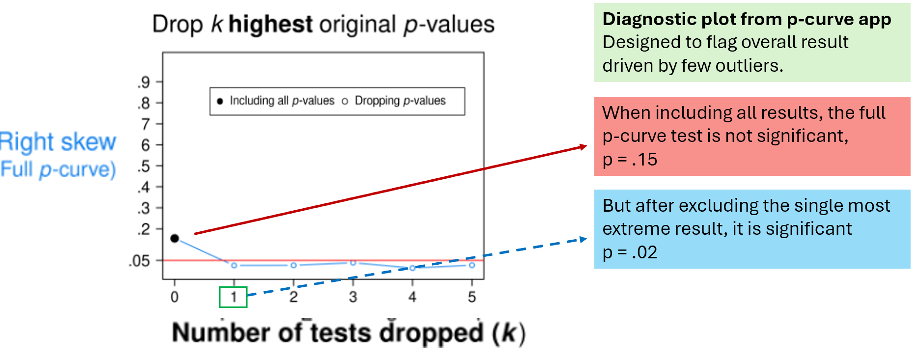
Figure 3. p-curve's diagnostic tools diagnose results driven by a single extreme p-value.

The y-axis has the p-value from a right-skew test for evidential value.
The x-axis has the number of high p-values dropped from p-curve to compute it.
To orient yourself, start on the left, which shows what happens when you drop none of the p-values. The full p-curve result is non-significant (p=.15).

We know that's only because of that unlikely p=.04988 we piano-dropped into it.
And the plot shows the p-curve app knows it too.

As you move right to the next marker, we see how that result changes if we drop the highest p-value in p-curve: it becomes significant with just 1 drop. And as you move further right, you can see that it remains significant. Thus, the plot clearly tells us that we have a p-curve with a result overturned by a single extreme study.

Conclusions
To give advice to researchers on what tools to use, you need to consider realistic scenarios under which they may use those tools, consider what the alterantives to those tools are, and what the researchers' goals are.

Appendix 1. Criticism 3. Heterogeneity biases p-curve
Appendix 2. Criticism 4: The Stouffer method is "inadmissible"

Criticism 3: Heterogeneity biases p-curve's power estimate
The JASA paper proposes that p-curve's power estimator, under heterogeneity, is inconsistent. This means that no matter how many studies you include in p-curve, the power estimate will contain some bias. The paper does not quantify, however, how much bias to expect. Instead, a piano is dropped on a car; an unlikely edge-case is shown to lead to substantial bias. The authors then generalize this result to all possible scenarios writing (p.29):

"Any situation more complicated than a single [power level] will be effectively impossible for [p-curve]".
Big, if true.

In contrast to this claim, in DataColada[67] "p-curve handles heterogeneity just fine", posted back in 2018, we show that under scenarios of very substantial heterogeneity, p-curve recovers average power with minimal if any bias. What we did was simulate large numbers of studies with a sample size chosen at random, true effect size given to the study at random, resulting in a random level of power. Then we considered a p-curver submitting the subset of studies that are significant to p-curve and trying to recover the true average power of the underlying studies.

We show the results with figures like the one below. We see ample variation in sample size and effect size, leading to ample variation in power, AKA heterogeneity. And yet p-curve's estimate is off by about 1%.

The JASA authors cite this blogpost and propose that in it, we didn't realize p-curve could be biased, they write: "[this blogpost's] argument was based only on seven simulations . . . they simply did not find a simulation violating their intuition" (p.30).

One problem is that we had nine, not seven simulations.
A bigger problem is that that shrouded eighth simulation involves, contrary to the quoted text above, a scenario where p-curve is biased.
An even bigger problem is that that eighth scenario is awfully similar to the scenario in the JASA paper, the one supposedly contradicting our analyses.

Call me old-fashioned, but I would have expected that someone using the scenario on the left would credit the people using the scenario on the right, and not, instead, explicitly claim the people on the right never thought of a scenario like the one on the left.

OK. That's the 8th simulation in our post. What about the other simulation they told readers did not exist? The 9th simulation in our post? It is also rather relevant.

We use the 9th simulation to illustrate why we think that what's producing the bias is not heterogeneity, as Schimmack and others conjectured in 2018 (and Morey & Davis-Stober conjectured in 2025), but instead, the culprit is the presence of outliers, studies with very high power (e.g., 99%+ power). In that 9^th simulation we considered a distribution of power across studies with a similar level of heterogeneity, but without outliers. p-curve did fine.

Criticism 4: The Stouffer method p-curve uses in "inadmissible"
There are two commonly used methods for combining p-values, Fisher's and Stouffer's.
Our original p-curve paper used Fisher, but shortly after publishing it, when writing a follow-up paper, "Better p-curves" (htm), we switched to Stouffer.

The JASA paper points out that a paper by Marden (1982), showed that the Stouffer method is "inadmissible".

This is one of those cases where statisticians choose a word to describe a statistical property that has little to do with how the word is used outside of statistics.

When Marden deemed Stouffer "inadmissible" (a term that already existed), he didn't mean that Stouffer provides results that ought to be ignored, or results that are illegitimate or invalid. Instead, "inadmissible” simply means that there could exist another method that is equally powerful, or more powerful than Stouffer’s, for every possible scenario.

So, a more accurate term, instead of "inadmissible test", might be "submaximal-power test".

In practice, Stouffer has very similar power to Fisher. For example, when shifting to Stouffer we redid all the simulations we had previously done with Fisher in our p-curve paper, the biggest power drop was 2%, and most power levels were effectively identical (pdf).

All else equal we would of course choose the method with higher power, Fisher over Stouffer. But all else is not equal. Stouffer has three properties that are appealing in the context of p-curve analysis:

Property 1 that makes Stouffer appealing
Stouffer is less sensitive to individual extreme p-values, but more sensitive to several moderately low values.

For example, say you are p-curving 5 p-values.
If all five were p=.01s, moderately low, Stouffer gives you a stronger summary than Fisher.
p_stouffer= .03 vs p_fisher = .097.

But if one is super low, p=.000001, and the other four are high, say p=.045s, Fisher is stronger.
p_stouffer= .68 vs p_fisher= .012.

Once you consider the possibility of reporting errors, confounds, fraud, etc., it is more diagnostic of credibility to have multiple moderately low p-values than a single extremely low one, and thus, Stouffer's method places weights on evidence that we believe are more rationally justified once we accept that there are sources of error other than sampling error. Indeed, the power losses for Stouffer come from its lower sensitivity to extremely low p-values. So we would argue those power losses are a feature, not a bug.

Property 2 that makes Stouffer appealing
Stouffer provides symmetric evaluations for the left- and right-skew tests, so the p-value for the left-skew test is 1 – p-value for right-skew test. With Fisher you could possibly simultaneously conclude both that a p-curve is right-skew and left-skew (this could happen if you have an extremely low p-value and an extremely high p-value, e.g., .001 and .0498).

Property 3 that makes Stouffer appealing
Stouffer allows placing unequal weights on p-values. We ended up not exploring this, but we thought at the time this may allow including multiple results from the same study into p-curve (e.g. p-values for two alternative DVs). If we ever return to working on p-curve it's an avenue we would explore (and possibly quickly dismiss).

The small community of researchers citing Marden has made arguments similar to ours
According to the web-of-science, the paper by Marden (1982), the one pointing out the submaximal power of the Stouffer method, has been cited 24 times. I looked into what the most recent and most cited among those 24 papers say on this matter

The most cited paper among those 24 is by Rice (1990), with 187 citations. Rice argues against using Fisher when "asking whether a set of tests, on balance, supports or refutes a common null hypothesis". (p.303; bold added). By "on balance" Rice seems to mean that the overall result should ideally not be driven by a single very strong test, a sentiment very similar to our first argument for Stouffer. Indeed, Rice then notes that Stouffer is "not disproportionately sensitive to [single] tests that refute H_o" (p.305)

The most recent paper among those 24, published in JASA, is by Wang and Owen (2019), who make a similar argument against an overall rejection conclusion that's based on a single extreme test. They write "thus it is possible that the null is then rejected largely on the basis of just one extremely significant … test. Such a rejection may be undesirable as it could arise from some irreproducible property of the setting in which that one … test was made. " (p.158, emphasis added. Note that they propose a new method that's neither Fisher's nor Stouffer's).

We are thus not alone in considering properties other than maximal power, other than "admissibility", for choosing statistical procedures.

References for Appendix 2.
Marden, J. I. (1982). Combining Independent Noncentral Chi Squared or F Tests. The Annals of Statistics, 10(1), 266-277.
Rice, W. R. (1990). A consensus combined P-value test and the family-wide significance of component tests. Biometrics, 303-308.
Wang, J., & Owen, A. B. (2019). Admissibility in partial conjunction testing. Journal of the American Statistical Association, 114(525), 158-168.

Feedback policy
Our policy is to contact authors whose work we cover to receive feedback before posting. I did not reach out to the authors of the JASA paper, Richard Morey and Clintin Davis-Stober, because they already made their paper public and I wanted to have a relatively timely response. FWIW, I had asked them to share the paper with me before they made it public, so that I could provide feedback and we could have a private dialogue. But they refused. In my fourth and last request for the paper I outlined 7 'pros' and 1 'cons' to sharing the paper. I list them in this footnote in case someone finds those arguments useful. [5]

Subscribe to Blog via Email

Footnotes.

Receipts for "long have been recognized".
Two of the four properties (monotonicity violations & impact of outliers) motivated design decisions of our p-curve app back in 2014 & 2015, such as communicating the # of p>.05 results excluded from p-curve, reporting robustness results excluding extreme p-values, and switching to the Stouffer method so as to be less sensitive to p-values that were extremely low or extremely close to .05. We did pay less if any attention to the issue specifically at the .025 cutoff, and the JASA paper focuses on that cutoff for some examples. In terms of the third criticism, Stouffer having lower power than Fisher, when we made the switch in our app, from Fisher to Stouffer, we redid all simulations from our published paper and reported (modest) drops in power with Stouffer. But we were unaware of Marden's (1982) general proof of Stouffer not having maximal power. In terms of the fourth criticism, that heterogeneity biases p-curve, it was made by a few authors back in 2018, and we responded to it sixty-two blogposts ago: in https://datacolada.org/67.

[↩]
Mixed models can violate monotonicity.
Here is the intuition:
Mixed-models assume a symmetric distribution of effects and so when it sees a Stimulus #10 with a very big effect, it says "shoot, there probably is another stimulus just as far from the mean but to the other side of it" and so, while the mean estimate goes up, the SE goes up more, turning it into a non-significant effect.

Here is the R Code with a concrete llustration

[↩]
Number of simulated studies in monotonicity simulations.
The text says I simulated 10 studies per simulation, but I actually simulate 10 in expectation, with substantial variation across simulations. Specifically I draw 10 over the power level of the studies (e.g., draw 20 studies when using 50% power). I then keep the subset that is significant. For the 35% power simulations, for example, the number of simulated studies in p-curve ranged from 5 to 20. The results are indistinguishable to the naked eye when always drawing exactly 10 significant studies per p-curve
[↩]
Why p=.0498?
I figured out what's the highest possible p-value you can get with a t-test reported to 3 decimal values, with n=100 per cell, and it is t(198)=1.972, p=0.04988.

[↩]
Pros and Cons of sharing critiques in advance
On my last email to Clintin, which did not prompt a reply, I wrote the following pros and cons of sharing the paper with us.

<email quoted text starts>
Here is how i see the pros and cons of sharing ahead of time:

Pros.
1. It's the mensch thing to do, ask any non-academic friend, they will tell you it is rude not to. Ask any academic friend, they will be surprised we have not seen it yet, that we were not reviewers. I have shown through revealed preference I deeply believe in sharing ahead of time (it's our policy at our blog Data Colada)

2. As hard as it may be to accept it, it is possible you have errors, my expertise and experience may help you spot them before the document is public

3. Maybe easier to accept, you may be communicating things in ways that are not perceived as you intend, idem. (as we say in our policy, i can help you spot things that are "snarky, inaccurate or misleading").

4. Related to 1, without sharing in advance, you take control over my time, whenever you decide to post the paper i have to allocate my time on that instant to your document, or pay the cost of not participating in the debate when people are paying attention to it. With two weeks notice, i have some ability to prioritize and some time to think things through before expressing ideas.

5. For the audience, the most important party, it's always better to see argument and counter-argument jointly so they can make up their minds with all the information

6. It's crazy we were not invited as reviewers of this paper, counter normative to how many journals operate, it's a conciliatory act to make up for that

7. Not sharing it may become a distraction if that becomes part of the conversation instead of the substance.

Cons.
1. You add 2 weeks to the multi year process of preparing the paper for public consumption (I think Richard started thinking about p-curve some 7 years ago at least).

So, i don't think it's a close call.

Uri

</email ends>
[↩]

Subscribe to Blog via Email

Related