Just two steps are needed to go from computing p-values to computing Bayes factors. This post explains both steps and introduces Hyp-Chart, the missing link we arrive at if we take only the first step. Hyp-Chart is a graph that shows how well the data fit the null vs. every possible alternative hypothesis [1].
Hyp-Chart may be useful for understanding evidence.
Hyp-Chart is certainly useful for understanding Bayes factors.
Hyp-Chart is also useful for conveying why I do not use Bayes factors in my research.
Hyp-Chart, the graph, is not new, I suspect many people have drawn it when teaching Bayes factors, but it did not seem to have a name, and it needed one for this post [2].
R Code to reproduce all figures in this post
Starting point: the p-value
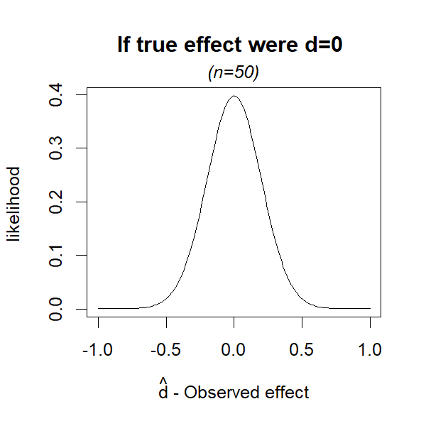
To compute a p-value we ask: if the null hypothesis were true, how likely is an outcome at least as extreme as the one we observe? To compute that, we need the likelihood of every possible outcome if the null were true (dtrue=0). Figure 1, which you’ve seen a million times, depicts those likelihoods.
Unfamiliar with d as measure of effect size? See this footnote [3].
Fig 1. If null is true, dtrue=0, what’s the likelihood of each estimate?
So, say you run a study and get d̂ =.5. The likelihood of that estimate under the null of dtrue=0, is found in that distribution. Specifically, it’s represented by the small vertical red line in Figure 2.
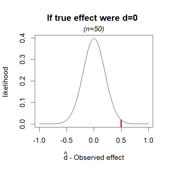 Fig 2. If null is true, dtrue=0, how likely is d̂ =.5?
The p-value is the probability of getting an effect at least as extreme, so the area to the right of that red line (for a one-sided test). But for this post we will just focus on the red line itself. With this review behind us, let’s now get to the two steps required to get a Bayes factor instead of a p-value.
Step 1: Compute likelihood of alternative hypotheses
A sensible criticism of how some people use p-values, is that they, the people, focus exclusively on the null and not on alternative hypotheses. If the null is false, what is true instead?
Figures 1 & 2 showed us what to expect if dtrue=0. Let’s now make new figures with what to expect if dtrue ≠ 0, that is, if the null is false. Let’s start with the alternative that the effect is “Medium” (dtrue=.5).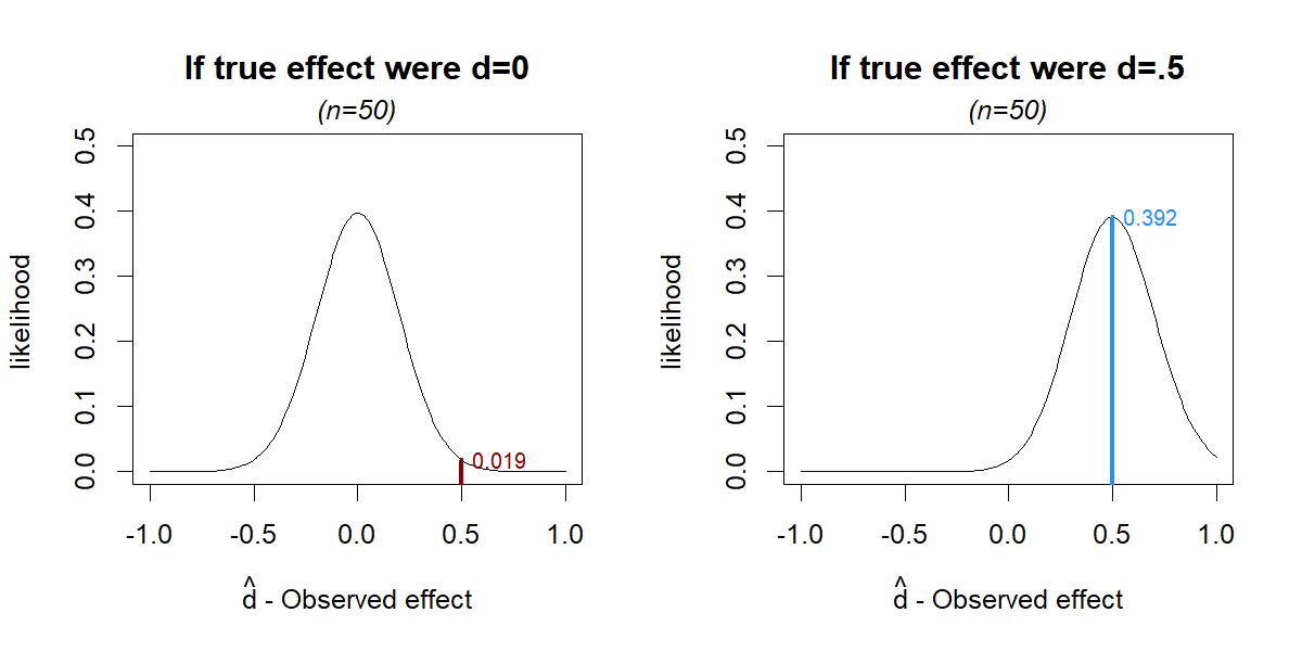
Fig 3. How likely is =.5 under dtrue=0 vs dtrue=.5
[the left chart is Figure 2 again]
We see that if dtrue=.5, getting d̂=.5 is more likely than if dtrue=0. That makes sense. If the effect is indeed bigger, it is more likely that we will estimate it as bigger.
We can quantify how much more likely d̂=.5 is under the alternative, by dividing the long vertical line in Figure 3, by the short vertical line. We get 0.392/0.019=21. That number, 21, is called the “likelihood ratio”, because it is a ratio, of likelihoods: it tells you that d̂=.5 is 21 times more likely if dtrue=.5 than if dtrue=0
Ok. But, what if the effect were Small (dtrue=.2) or Large (dtrue=.8) instead of Medium?
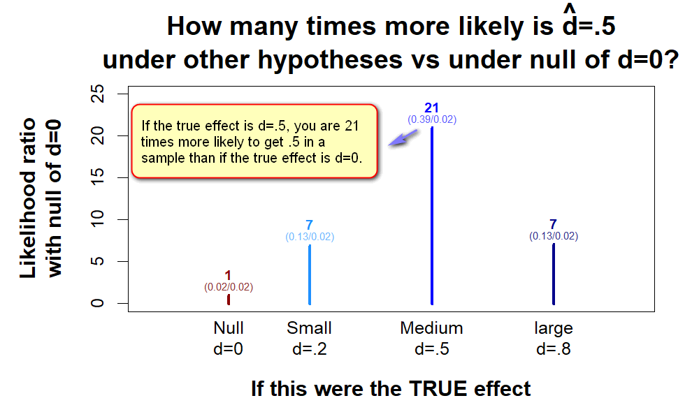
Fig 4. How likely is d̂ =.5 if dtrue=0 vs if it is Small, Medium or Large?
We can do this for every possible hypothesis in a graph that I will (affectionately) refer to as ‘Hyp-Chart’.
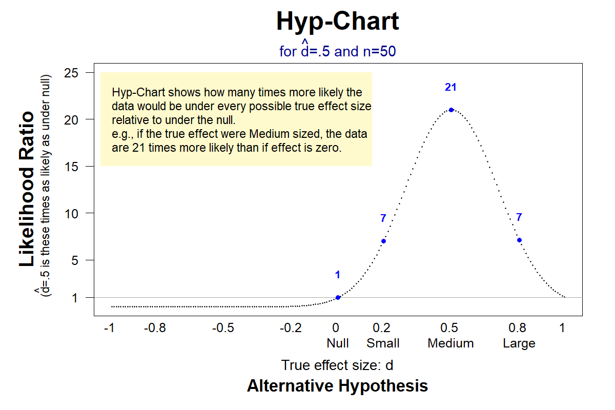 Fig 5. How much more likely is d̂ =.5, for every possible effect, than for dtrue=0?
Getting a feel for Hyp-Chart
The motivation for going beyond p-values, remember, was to look at alternative hypotheses, and not just the null hypothesis. To illustrate how Hyp-Chart achieves this, Figure 6 depicts Hyp-Charts for the same p-value, p=.02, but different sample sizes (n=100 vs n=500), and thus different observed effect sizes ( d̂ =.33 & d̂ =.15).
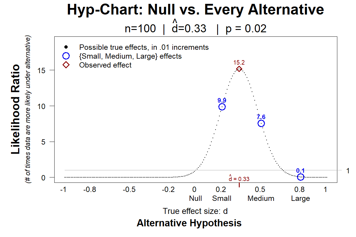
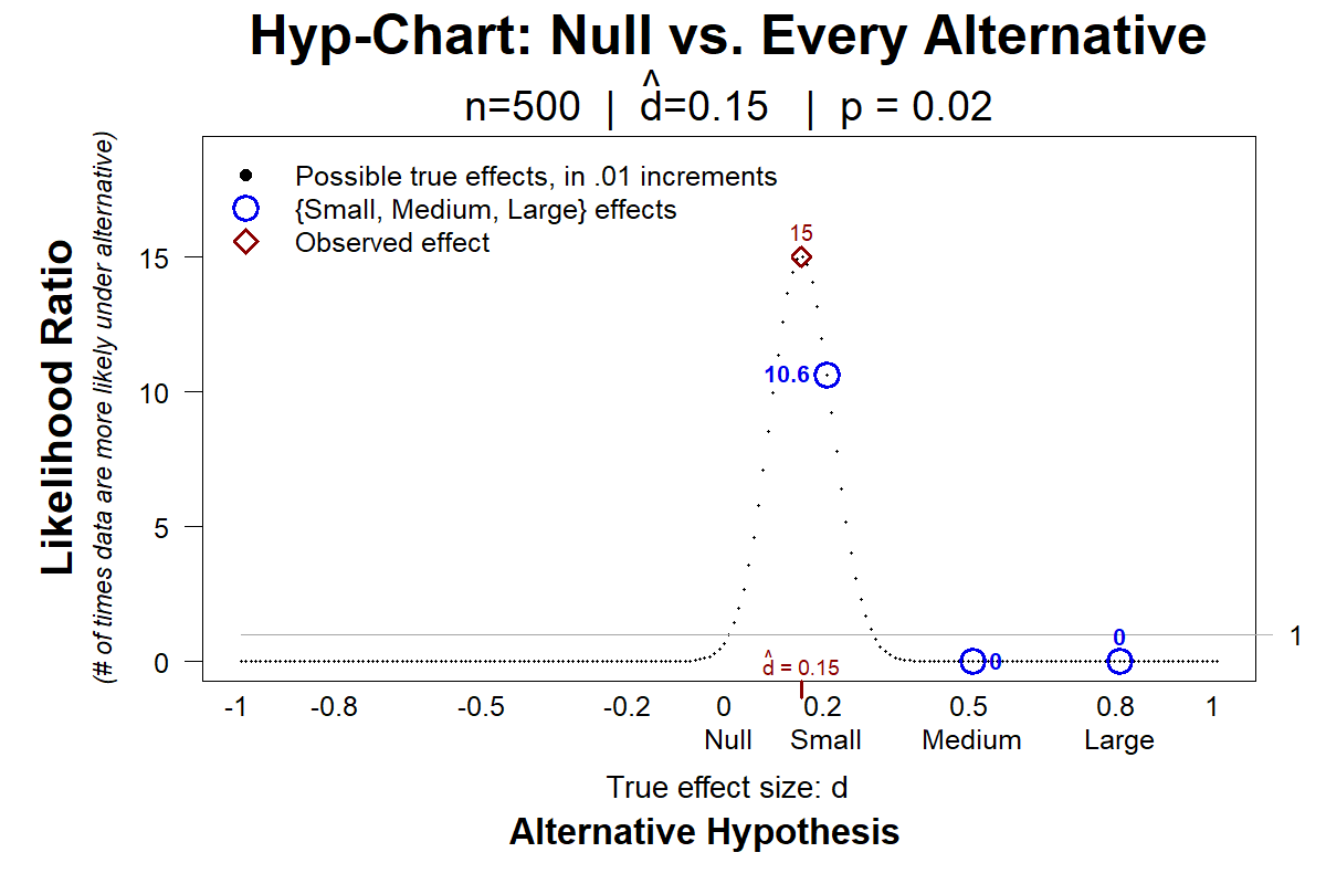
Fig 6. Hyp-Charts for p=.02 results, with n=100 vs n=500
Both studies reject the null equally strongly, p=.02, but they tell us different things about the alternative. For example, on top, the data are 7.6 times more consistent with a Medium effect than with the null, but in the bottom the data are not at all compatible with a Medium effect.
Interlude
This first step from p-value to Bayes factors, Hyp-Chart, is neat and seems to convey interesting information about alternative hypotheses. I personally prefer confidence intervals, but reasonable people could disagree with me and prefer Hyp-Chart over, or in addition to, confidence intervals (one could add the confidence interval to the x-axis of the Hyp-Chart).
In contrast, it does not seem reasonable for social scientists at least, to go further, to take the second step, and compute a Bayes factor. OK. Let's see what that second step is.
Step 2: The Bayes factor is a (bad) summary of Hyp-Chart
Like Hyp-Charts, Bayes factors compare the likelihood of the data under the null vs “the alternative”. What's different is that instead of reporting results for each possible effect, the Bayes factor reports only one number, a single (weighted) average across all the likelihoods in Hyp-Chart. [4].
Figure 7 below illustrates how default Bayes factors average a Hyp-Chart to evaluate “the alternative”.
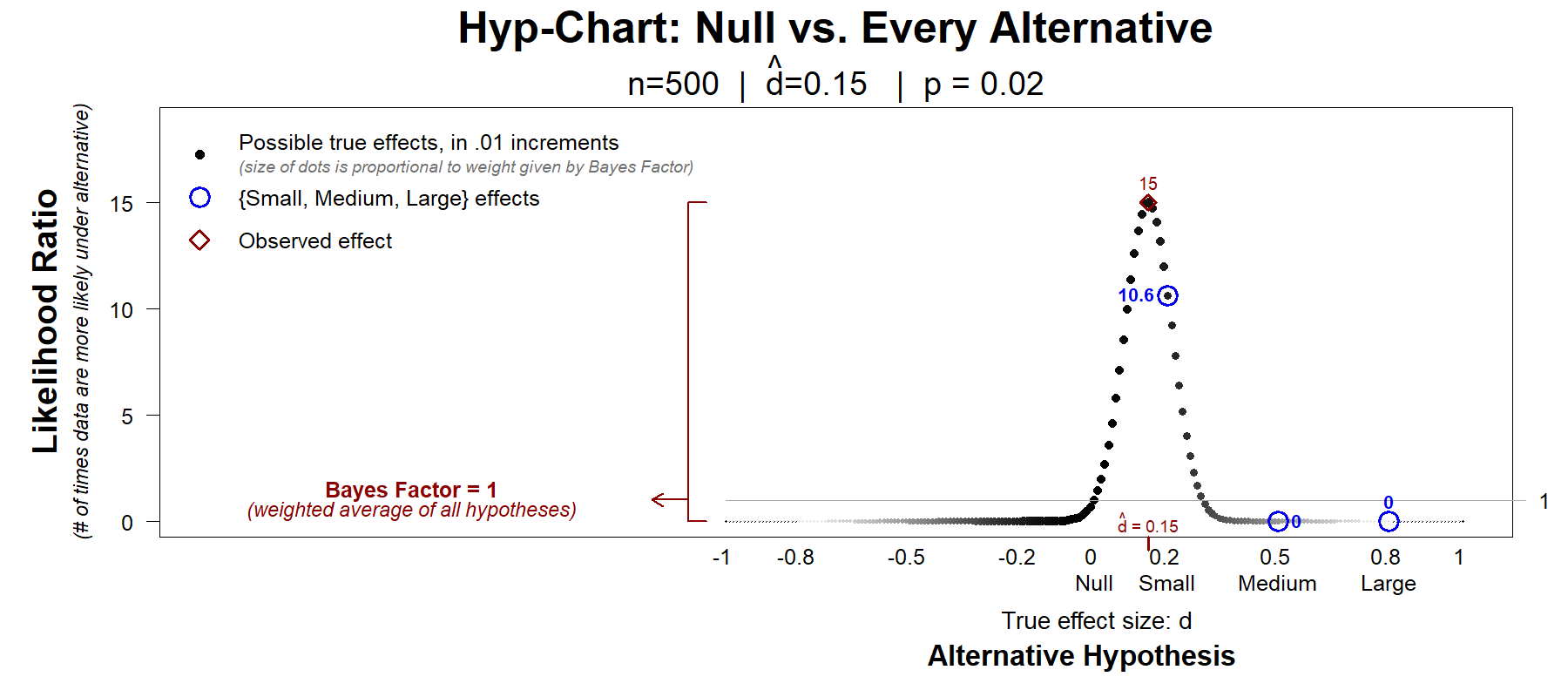
Fig 7. A Bayes factor vs its underlying Hyp-Chart
The figure is just like the previous Figure 6, but the size of the dots is proportional to the weight given by the default Bayes factor.
The weighted average is BF=1. The Bayes factor, then, summarizes the above Hyp-Chart by saying that the null and ‘the alternative’ are equally consistent with the data. That d̂ =.15 is just as likely if dtrue=0 as if "the alternative" is true.
But the Hyp-Chart shows that the data are 11 times more consistent with a small effect, dtrue=.2, than with the null of dtrue=0. 15 times more consistent with the observed effect of dtrue = .15 than with the null. That is relatively strong support for true effects that in many contexts are large enough to be of interest.
I doubt many (any?) readers of a paper that reports “BF=1”, that reads “the null is as consistent with the data as with ‘the alternative’”, or that reads “the data are non-diagnostic from a Bayesian standpoint”, would imagine that the data are 11 times more consistent with a small effect than with zero.
Bayes factors change their mind about what ‘the alternative’ is.
Hyp-Chart helps convey another reason why I don’t use Bayes factors
With default Bayes Factors: every effect size estimate that ‘supports the null’ for one sample size, ‘supports the alternative’ for a larger sample size [5].
This is not something Bayesian advocates don’t know. But it is something that does not bother them [6], and that I think would bother most social scientists.
To illustrate, let’s consider the observed d̂=.15 we have used a few times.
If you run a study with n=150, and get d̂=.15, the Bayes factor will favor the null
If you run a study with n=750, and get d̂=.15, the Bayes factor will favor the alternative
This is NOT the same as d̂= .15 being statistically significant only for big n.
It is one thing to go from “don’t know” to “x is false", as p-values do. It is another to go from “x is true” to “x is false”, as Bayes factors do.
Let’s dive deeper into these two scenarios, this time aided by Hyp-Charts.
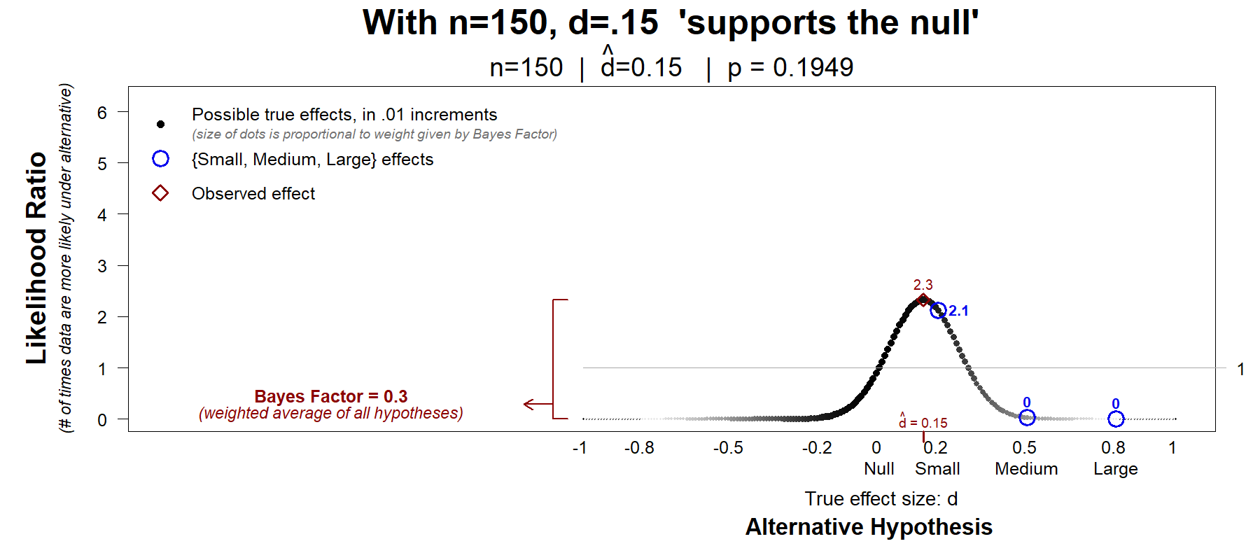
Fig. 8. Bayes Factor is BF < 1/3, so we conclude d̂ =.15 supports the null
Getting d̂=.15 with just n=150 is an inconclusive result, for sure, note that p=.19 after all. But that result is 2.1 times more consistent with a small effect of d=.2 than with the null. The Bayes factor, however, does not call this study inconclusive. After averaging that 2.1 with lots of 0s from hypotheses with the opposite sign, and hypotheses for quite large effects – hypotheses we have no specific reason to expect or predict or care about – it computes a low average, a low Bayes factor, BF<1/3, so d̂=.15 “supports the null”.
The conclusion reverses, for the same result, d̂=.15, with a larger sample,
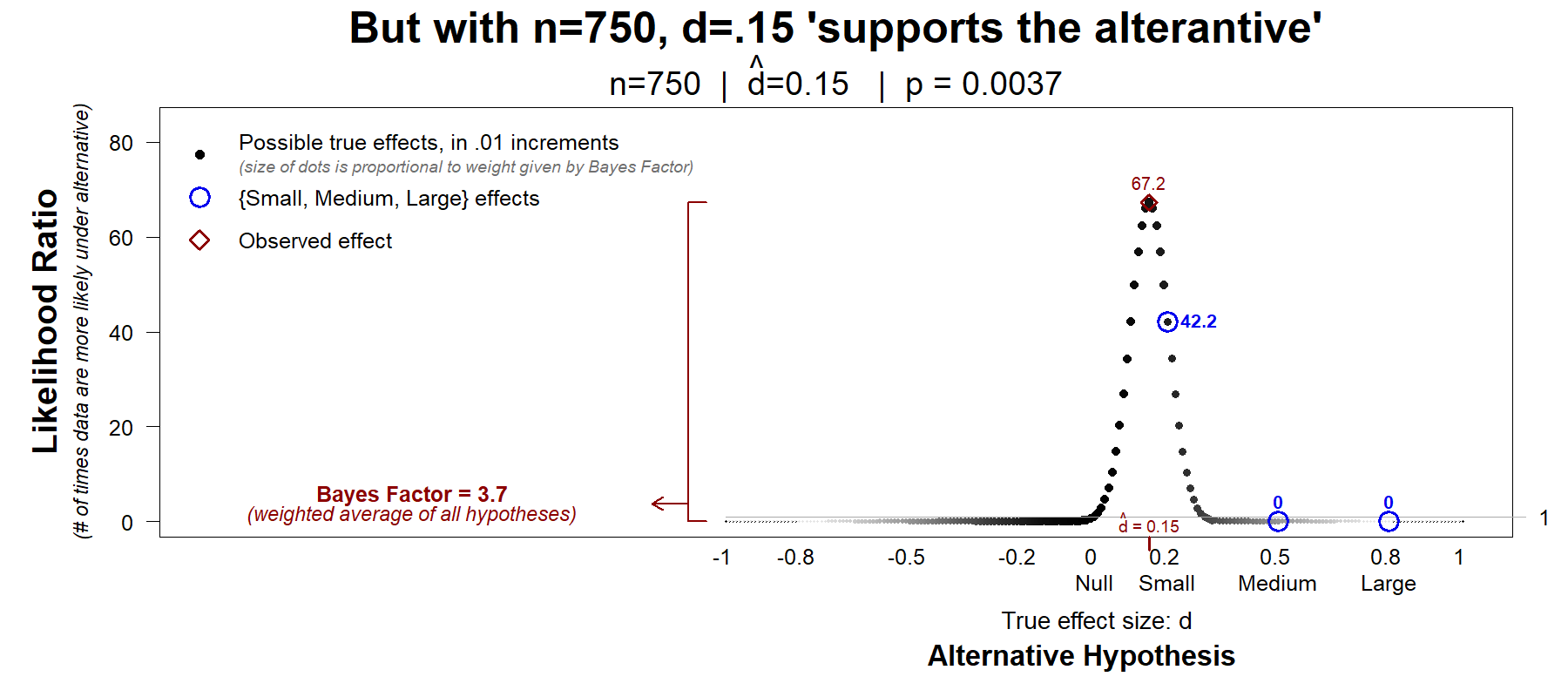 Fig. 9. Bayes Factor is BF > 3, so we conclude =.15 supports ‘the alternative’
The Bayes factor does now give a qualitatively sensible summary of Hyp-Chart. But as a quantitative summary, the Bayes factor seems misleading. The observed value, BF=3.7, means the data are 3.7 times more consistent with ‘the alternative’. But the data are 42 times more compatible with a small effect than with a null effect, and 67 times more compatible with the observed effect than with a null effect.
Run these two lines of R Code to make your own Hyp-Charts
source("http://webstimate.org/hyp-chart/Hyp-Chart_2019_09_05.R") #Load the Hyp-Chart function
hyp.chart(d.obs=.4, n=50, show.bayes=TRUE) #Set n (per-cell sample) and either observed effect (d.obs) or p-value (p.obs)
Take home.
Reporting a Bayes factor seems like an unnecessary reduction, and distortion, of the available information contained in a Hyp-Chart. If you review a paper that reports a Bayes factor, I recommend you ask the authors to include a Hyp-Chart alongside it. This will allow readers to interpret the data using their actual prior beliefs and actual theories of interest, instead of using the (irrelevant) average prediction, made by a default hypothesis they don't hold (or understand).
This is the second post in the Bayes factors series, see the first: Colada[78A]
![]()
Feedback
I shared a draft of this post with Felix Schönbrodt (.htm), and Leonhard Held (.htm) who have written on Bayes factors in the context of hypothesis testing, and with Bence Palfi (@bence_palfi), a PhD student from Essex who had identified an imprecision/error in my previous post (Colada[78a]). A parallel conversation with Zoltan Dienes (.htm), following that post was also useful. They were all polite, respectful, and helpful, despite having different summary evaluations of the usefulness of Bayes factors. Thanks.
Footnotes.
- Technically speaking, every alternative hypothesis involving a "degenerate distribution", which just means hypotheses over single values, e.g., that dtrue=.45 [↩]
- Alex Etz (.htm) complained that I'd propose a new name, "Hyp-Chart", for what is 'just' a re-scaled likelihood function. Hyp-Chart is indeed a likelihood function, but where we know what's in the x-axis, the candidate hypotheses fed into a Bayes factor, and more importantly, the y-axis, the ratio with respect to the likelihood of the null. You can see Alex's tweet (.htm), and his previous relevant writing on likelihoods published in AMPPS .htm and his previous blog post with similar content .htm [↩]
- Throughout I use Cohen’s d as a measure of effect size. When comparing two means, d is the difference in means divided by the standard deviation. d=(M1-M2)/SD. I use dtrue to symbolize the different in population means, and d̂ for the estimated difference [↩]
- In principle Bayes factors can combine any subset of alternative effects (including just one), and in principle Bayes factors can weigh them in any way. But, in practice, Bayes factors are computed using hard-coded default “alternative hypotheses” which give a pre-specified weight to every effect, of both signs, giving much more weight to dtrue’s near zero. The defaults are either that d~N(0,.7) or a JZS prior. The distinction is not relevant for this post. Indeed, I plot the Hyp-Charts using the former but compute Bayes factors using the latter [↩]
- The sole exception is d̂=0. An exact zero estimate, never supports the alternative. Then again, exact zeros are impossible [↩]
- Bayesian advocates probably would not even agree with my characterization that the same point estimate supporting the null and then supporting the alternative involves a "change of mind", they would just see it as the natural consequence of a likelihood function for two different sample sizes. But my guess is that for most social scientists, an observed d̂ =.15 cannot simultaneously support and oppose the same theory. The math behind the Bayes factor is correct, but, in my view, it poorly captures how researchers think and want to think about evidence. [↩]
