[102] R on Steroids: Running WAY faster simulations in R

This post shows how to run simulations (loops) in R that can go 50 times faster than the default approach of running code like: for (k in 1:100) on your laptop. Obviously, a bit of a niche post.

There are two steps.

Step 1 involves running parallel rather than sequential loops [1].
This step can increase your speed about 8 fold.

Step 2 involves using a virtual computer instead of your lame laptop.
This step can increase speed about another 7 fold.

Both steps combined, then, lead to about 50 fold speed increase [2].

If you already know how to run parallel loops on a virtual desktop, check out step 2 anyway, it suggests a faster, simpler, cheaper, more flexible alternative to Amazon's AWS.

A motivating example: simulation to evaluate whether likert scales can be t-tested
To have a concrete loop to contrast sequential vs parallel, let’s consider running simulations to see if it is OK to run a t-test on a likert scale. Specifically, the simulation generates two random samples with possible Likert values (1, 2, 3, 4 or 5), runs a t-test on these two samples, and saves the p-value. The loops repeat this simulation 8000 times, saving the p-value each time. Once all the simulations are completed, we can check how many of these p-values are smaller than .05 (should be 5%). This example is good in that it is simple and at least somewhat interesting, but the example is bad in that the simulation is not very demanding so it runs fast enough without bothering with parallel processing. This code runs in seconds. But more demanding simulation can take hours to run. In any case, the simulation would be like this:

set.seed(111)
p=c()
for (k in 1:8000) {
x1=sample(1:5 , size=30,replace=TRUE)
x2=sample(1:5 , size=30,replace=TRUE)
p[k]=t.test(x1,x2)$p.value
}

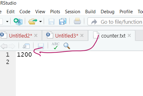
The loop produces a vector with 8000 p-values. The false-positive rate is the % of those 8000 that are p<.05. We can compute it with sum(p<.05)/8000. We obtain 4.94%. Close enough to 5%. So, turns out t-testing likert scales is fine [3].

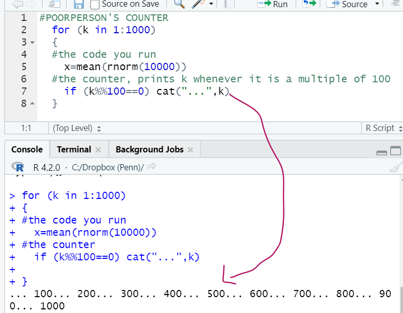
for() is kind of a dumb loop.
Dumb in that while our computers have the capacity to do many things at the same time, we are asking it to do only one thing, one loop, at a time. Computers come with multiple core processors. To know how many your computer has you can run parallel::detectCores()

My computer has 8. But I only used 1 to learn about likert scales above.
One of my 8 processors run 8000 simulations, the other 7 did nothing.

Imagine you visit a French restaurant with your favorite cousin. The waiter takes forever to come take your order, you are getting upset till you realize there is only one waiter working. But then, you realize there are 7 other waiters, all on break. You become upset again, and quickly come up with an idea that would speed things up.

Fig 1. Visual approximation of laptop while running a for() loop

That’s right. Have all the waiters instead of only one of them do some work.

Same with R, let’s have each of the 8 cores do 1000 simulations, at the same time, instead of one core do 8000 one after the other.

Step 1. Running parallel loops in R
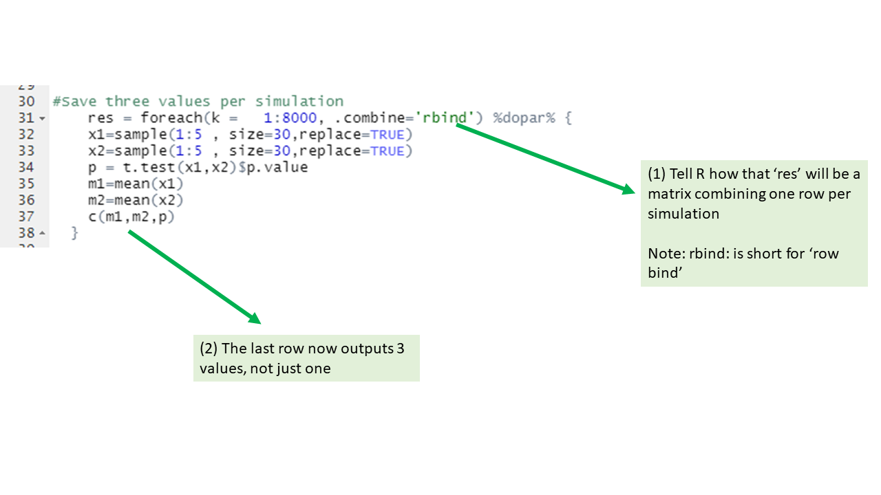
The figure below has annotated code for running the same loop we saw above, but in parallel.

#load packages
library('groundhog')
pkgs=c('foreach','doParallel')
groundhog.library(pkgs,'2022-07-01')

#get the core processors ready to go
registerDoParallel(cores=7) #I leave 1 free to do things while R runs

#Actual loop
p = foreach(k = 1:8000, .combine='c') %dopar% {
x1=sample(1:5 , size=30,replace=TRUE)
x2=sample(1:5 , size=30,replace=TRUE)
p = t.test(x1,x2)$p.value
p
}

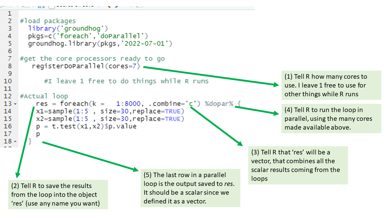
This loop will run about 8 times faster than the for() loop, minus the fixed time cost of setting up all the parallel processing. For fast tasks, parallel processing is not worth it.

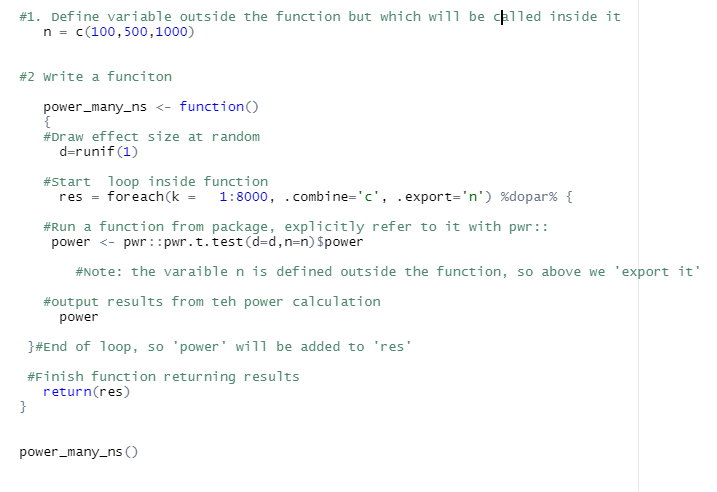
Intermediate level tips
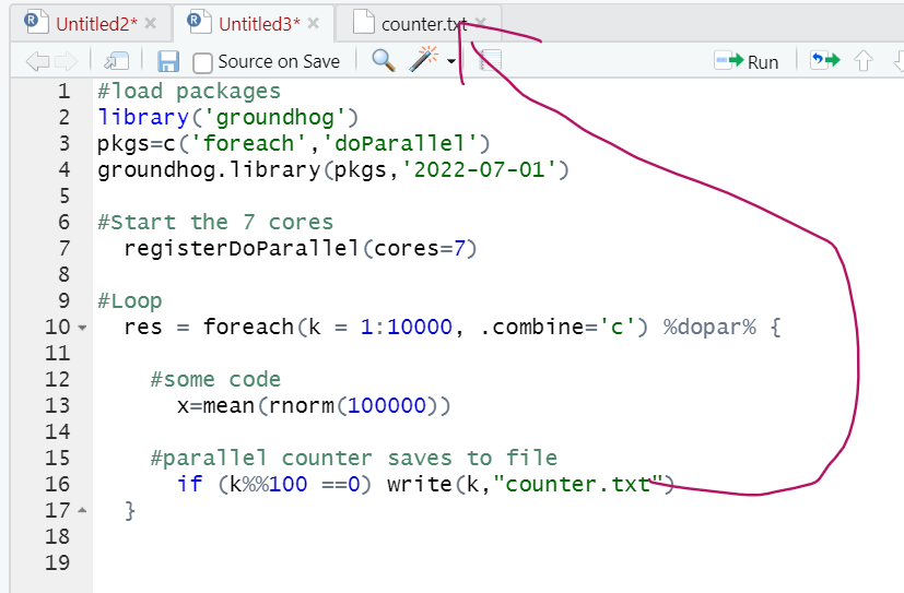
If you start using parallel loops, these extra pieces of info may be useful

1. Saving more than 1 number in every loop (e.g., a vector with 5 results)

The example above saves only one result per loop, one p-value. We often want to save many numbers after each loop, for example, we may want to save the means, the t-value and the p-value. You can do that by having the result of each loop be a vector instead of a scalar. To be able to do that the only thing we change is the .combine option. Instead of .combine='c', which tells R to use the c() function to put all the numbers the loops output into a vector, we use .combine='rbind' to tell R to use the rbind()function to put all resulting vectors produced by the loops stacked up vertically in a matrix.

The example below produces a matrix, where the first two column have 8000 means each, and the third column 8000 p-values.

Fig 3. Parallel loop saving a row of data in every loop

One may also save more complex sets of reults per loop, not just scalars and vectors. For example you can save an entire data-frame or a list. For that one can use what is actually the default for foreach loops, which is to save the result of each loop as an item on a list.

2. Using functions from packages inside parallel loops

If inside your loop you have a function that is from a package, say the function `pwr.t.test` from the ‘pwr’ package, make sure to include the package name in the call.

So instead of putting this inside the loop:
pwr.t.test(n=20, d=.5), you put this:
pwr::pwr.t.test(n=20,d=.5)

The reason is that the packages you load with ‘library’ or ‘groundhog.library’ are not sent to the parallel processors, so you need tell R running in those other processors where to find pwr.t.test [4].

3. Creating a function that has a parallel loop inside it

I often run montecarlo simulations from within a custom function, and inside that function I put the parallel loop. So the code looks like this:

montecarlo_function <- function(N) {

res=foreach(…{… yada yada yada )
}
return(res) }

If you have any objects that are referenced in that function (e.g., other functions written on that script), they will not be sent to the parallel cores and you will get an error when your code executes, for a called on function will not be found. So you just need to tell R to send those other objects to every parallel processor.

See the example below, where a variable created outside the custom function, the vector n=c(100,500,1000), is explicitly referenced in the foreach(), with the .export() option, so that it is sent to the parallel processors.

If you delete the `.export=’n’ option, you will get an error saying 'n’ was not found by the parallel processors. If you delete the pwr:: from pwr.t.test, you will get an error saying that the function pwr.t.test does not exist.

Fig 4. Intermediate level parallel loops. Putting loop in a function, and calling functions from packages

4. Showing a counter (to see how many loops have been done)

With serial loops I always use a simple counter that prints on the console the loop # every, say, 100 loops.

With parallel loops that will not work, because every parallel processor has its own instance of R open.
Instead, I have a text file that is saved to from the script, and I open the text file in R Studio. Whichever processor now happens to run the simulation that is a multiple of 100 saves to that text file, and R Studio refreshes when the file is saved, showing the loop number overall.

Here is the code that saves to a text file counter (I opened the text file in R Studio so it is now a tab)

And here is what you see if you click on the counter tab, e.g., there I was 1200 loops in.

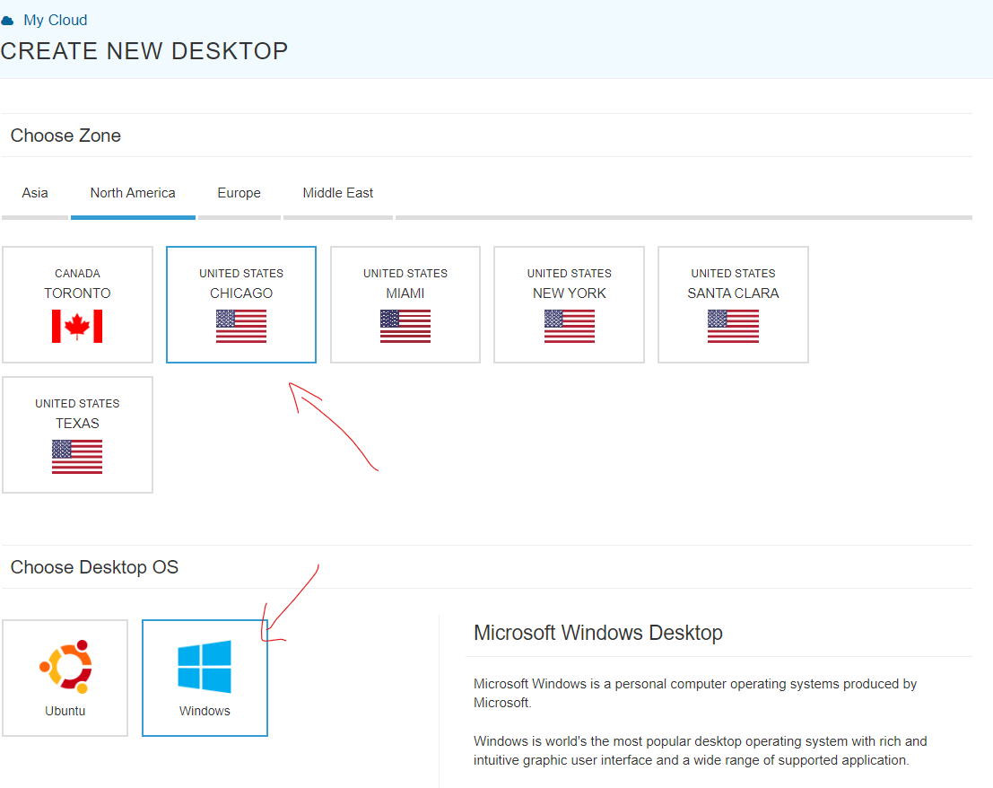
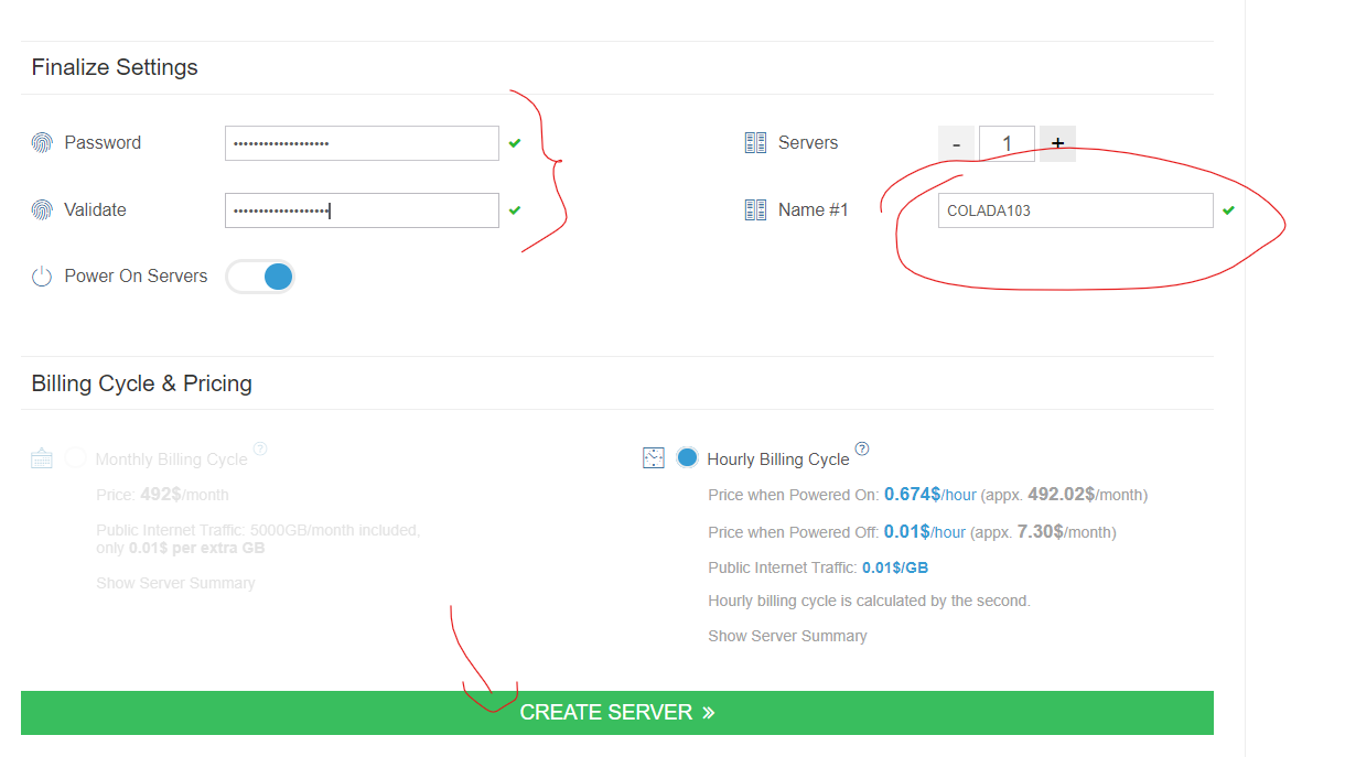
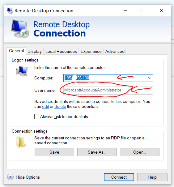
Step 2. Running parallel loops on a virtual desktop
Your laptop probably has at most 8 cores, limiting the benefits of parallel loops. If you run them on a virtual computer on the cloud with more cores, things will naturally go even faster. I will show you how to setup a virtual desktop with ~50 cores. You have to pay, but it is cheap, <$1 (one dollar) per hour of computations. I first used Amazon's AWS to run R on the cloud, but I recently came across a way better alternative kamatera.com.

If you haven't learned how to use AWS, do not bother.
If you have learned it, you probably will prefer Kamatera, it is much easier to use, way faster to set up, and flexible (e.g., you can easily update R and R Studio in it).

To use it, go to http://kamatera.com and then:

1. Create an account
(sorry, life is hard sometimes)

2. My cloud→Servers→Create New Desktop

3. Choose any location and presumably Windows machine.

4. Select the specs for your virtual computer
You probably want type=’burstable’

I am choosing 48 cores here, the key component, and some RAM and HD space which are usually not too relevant for loops.

Kamatera sets a limit to the specs based on how much it would cost to leave the virtual machine on for a full month. That limit is about $350. if you don't modify that cap (which you can do by emailing support) you will have to choose fewer than 50 cores. [5].

5 Choose a name and password for the virtual computer.

Note: Make sure to choose ‘hourly billing’ so you don’t get charged when you don’t use it

It takes about 5 literal minutes for the virtual computer to be created. So don't worry if it does not immediately appear.
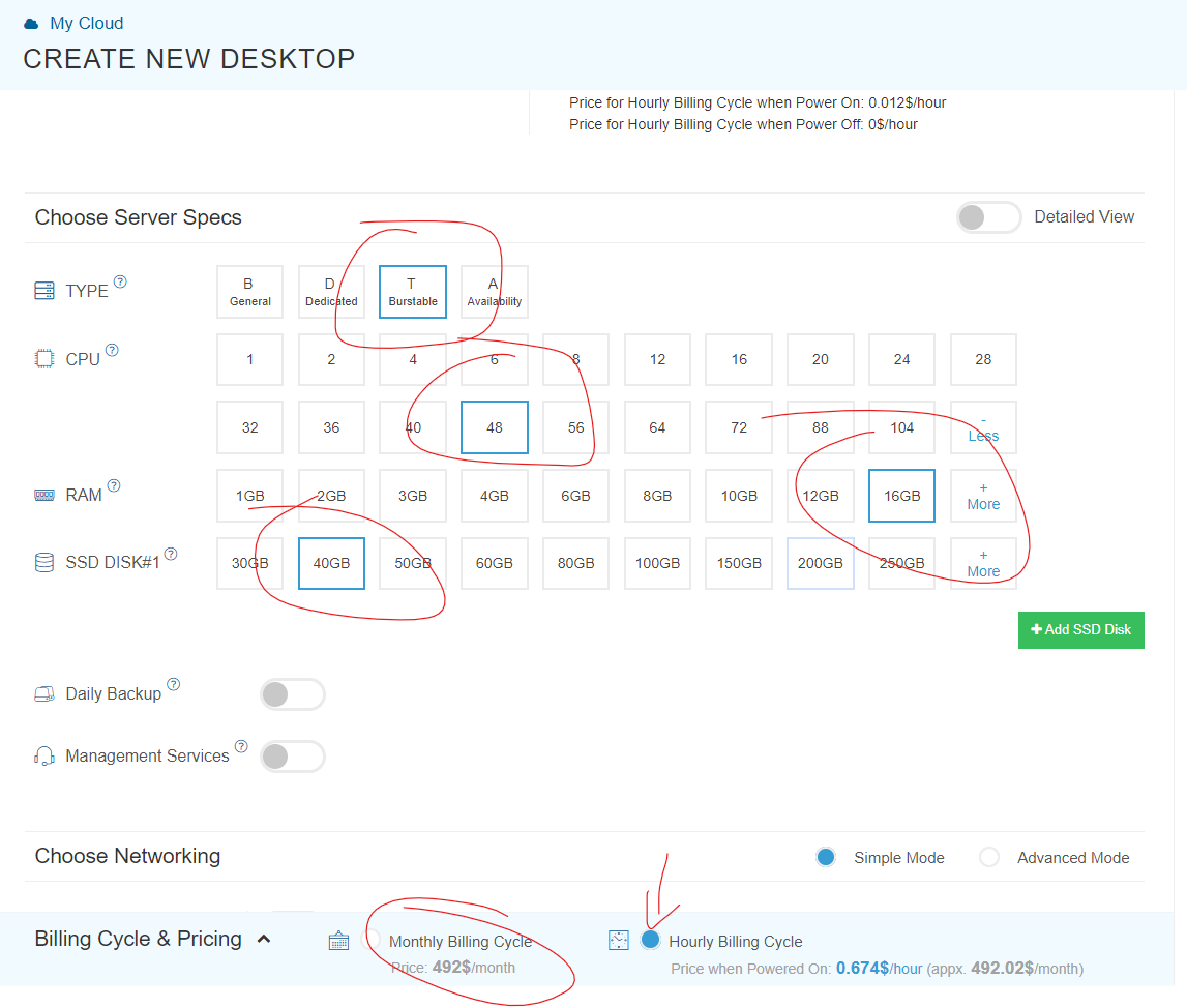
Kamatera actually emails you once they have it ready.

6. Then start the virtual computer clicking on “Action->power on”

7. Connect with remote desktop app in your computer, entering the IP address shown in the Kamatera site

Look at the arrow to see what to use as user name

Whem prompted for the password, enter the one you just set above.

Mac user? connect to the windows machine from your Mac with:
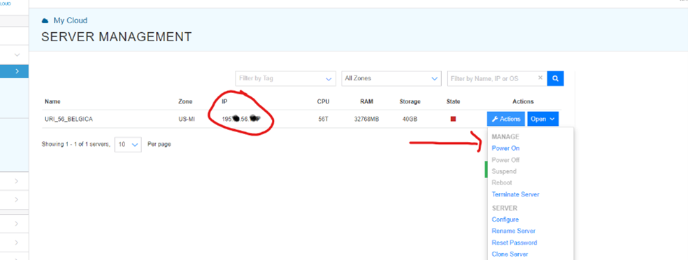
https://apps.apple.com/us/app/microsoft-remote-desktop/id1295203466?mt=12

8. Now you have a fully functional virtual windows machine.

Once you are connected this is your virtual machine, you can do everything in it you do on your pc. To install R Studio, for example, just open the browser and download it. You can also copy-paste code from your computer to the virtual one and vice versa.

9. Bonus: github
If you use github, that's by far the easiest way to send files back and forth. Install it in the virtual machine, and just pull before you work and push after you do. Code and results will be synced.

Subscribe to Blog via Email

Footnotes.

There are several blog posts and tutorials on running parallel loops (see e.g., blasbenito | esciencecenter | jbhender). I thought there was room for an attempt at a more intuitive and focused-on-simulations coverage [↩]
there are always fixed overhead cost, so not 56 times. Also, disclaimer: individual results may vary [↩]
This example only considered uniform distributions, but it is actually fine more generally [↩]
there are many ways to achieve this outcome, including the package name in the loop is by far the easiest [↩]
Note that as you change the specs the cost of keeping the machine on for the full month is displayed, and there default is a $350 cap, so you have to play around to get what you want and stick to under $350, or email support to get the cap increased. To be clear, you will spend WAY WAY less than $500, because that is the cost of keeping it on all month, you will probably use it for a few hours [↩]

Subscribe to Blog via Email

Related